Object Detection (Bounding Boxes and YOLO)

Classification gives one label per image. Segmentation gives one per pixel. Detection gives a variable number of boxes, each with a position, a size and a confidence — and that variability is the whole difficulty. A network outputs a fixed-shape tensor; the answer has a length the network cannot know in advance.

Every single-stage detector solves it the same way: divide the image into a grid and let each cell answer “is there an object centred in me, and if so, where exactly and how big?” This page builds that detector — 23,621 parameters, 2,000 synthetic 64×64 scenes, 18 epochs — and measures every part of it.

What you’ll learn

Why detection cannot use a fixed-length output, and the grid trick that makes it fixed anyway.
The five numbers per cell, and why every one of them is scaled into $[0, 1]$ .
Why the loss must mask the geometry terms by objectness — measured at 38.5× inflation when it doesn’t.
IoU as the only sensible “is this box correct” test: a 4-pixel shift on a 20-pixel box costs a third of it.
Non-max suppression, in five lines.
The measured trade: recall 0.8616 → 0.6799 as the objectness threshold rises 0.3 → 0.7, while precision sits still at ~0.997.

IoU first, because everything is scored with it

Two boxes are “the same box” only relative to a threshold on their intersection over union:

\text{IoU} = \frac{\text{area}(A \cap B)}{\text{area}(A) + \text{area}(B) - \text{area}(A \cap B)}

Case	Box A	Box B	IoU
identical	(10, 10, 30, 30)	(10, 10, 30, 30)	1.0000
shifted 4 px	(10, 10, 30, 30)	(14, 10, 34, 30)	0.6667
shifted 10 px	(10, 10, 30, 30)	(20, 10, 40, 30)	0.3333
half the size	(10, 10, 30, 30)	(10, 10, 20, 20)	0.2500
touching	(10, 10, 30, 30)	(30, 10, 50, 30)	0.0000
disjoint	(10, 10, 30, 30)	(40, 40, 60, 60)	0.0000

figure IoU for six box pairs matplotlib

The 4-pixel shift is the row to remember: a fifth of the box's width costs a third of the IoU. That is why 0.5 is called a lenient detection threshold and 0.75 a strict one, and why mAP@0.5 and mAP@0.5:0.95 are different sports. Note also that boxes which merely touch score exactly 0 — IoU has no notion of 'close'.

The grid encoding

The image is divided into an 8×8 grid of 8×8-pixel cells. Each cell predicts five numbers:

Number	Meaning	Range	Activation
objectness	is an object’s centre in this cell?	$[0, 1]$	sigmoid
$o_x, o_y$	centre offset inside the cell	$[0, 1]$	sigmoid
$w, h$	box size as a fraction of the image	$[0, 1]$	sigmoid

Encoding a box into a cell

def encode(boxes, grid=8, cell=8, side=64):
    target = np.zeros((grid, grid, 5), "float32")
    for x1, y1, x2, y2 in boxes:
        cx, cy = (x1 + x2) / 2, (y1 + y2) / 2
        column, row = min(int(cx // cell), grid - 1), min(int(cy // cell), grid - 1)
        target[row, column] = (1.0,
                               (cx - column * cell) / cell,   # offset in the cell
                               (cy - row * cell) / cell,
                               (x2 - x1) / side,              # size in the image
                               (y2 - y1) / side)
    return target

Both scalings exist for the same reason: every target lands in $[0, 1]$ , so a sigmoid can produce it. A network asked to regress raw pixel coordinates must learn the image size as well as the object, and it learns it badly.

The output is therefore $8 \times 8 \times 5 = 320$ numbers, fixed, whatever the scene contains. The encoding is exactly invertible — Exercise 2 round-trips two boxes with a maximum coordinate error of 0.00e+00.

diagram Diagram mermaid

  flowchart LR
  A["64x64 image"] --> B["conv stack
total stride 8"]
  B --> C["8x8x5 head
sigmoid"]
  C --> D["decode:
objectness > threshold"]
  D --> E["boxes in pixels"]
  E --> F["non-max suppression"]
  F --> G["final detections"]
  C -. "training" .-> H["masked loss:
objectness in every cell,
geometry only where an object is"]

The design’s built-in limit

One cell holds one object. Two centres in the same cell means the grid can only represent one of them — no loss function and no training budget fixes that. On this data it happens in 3.00% of scenes (Exercise 3). Real YOLO variants attach several anchor boxes per cell to raise the ceiling; a finer grid lowers the collision rate.

The imbalance, and the loss it forces

Quantity	Value
cells per scene	64
objects per scene (mean)	2.000
cells containing an object centre	0.0305
imbalance against a positive	32.8 : 1

A cell with no object still emits four geometry numbers, and those numbers are meaningless — there is no box for them to describe. The fix is one multiplication:

The masked loss

def detection_loss(y_true, y_pred):
    present = y_true[..., :1]                       # 1 where an object is centred
    objectness = keras.losses.binary_crossentropy(present, y_pred[..., :1])
    geometry = tf.reduce_sum(tf.square(y_true[..., 1:] - y_pred[..., 1:]), axis=-1)
    return tf.reduce_mean(objectness) + 5.0 * tf.reduce_mean(geometry * present[..., 0])

Objectness is scored everywhere — the model must learn where objects are not. Geometry is scored only where an object is. Exercise 6 measures the cost of getting this wrong on a 2×2 grid holding one object, with the model guessing 0.5 everywhere:

Geometry loss	Value
over every cell	0.770000
masked to cells with an object	0.020000
inflation from the three empty cells	38.50×

Thirty-eight times the loss, and every bit of the excess is the model being punished for box coordinates that describe nothing. The 5.0 weight on the geometry term exists for the opposite reason: one objectness term across 64 cells otherwise drowns out four geometry terms in one cell, and the model settles for saying “no object” everywhere.

What the trained detector does

23,621 parameters, 18 epochs, final loss 0.0210, validation loss 0.0239.

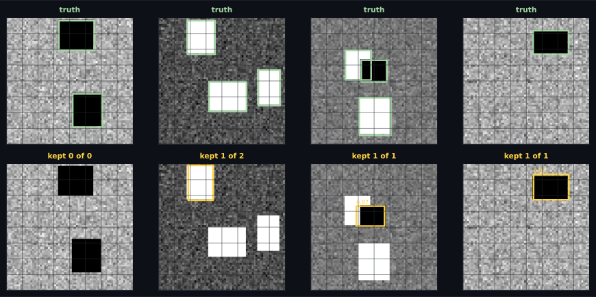
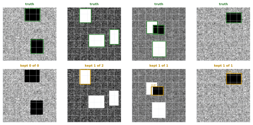
Two rows of four panels. The top row shows four test scenes with green ground-truth boxes over noisy grey backgrounds containing dark or light rectangles: two, three, three and one object. The bottom row shows the same scenes with kept detections in amber, labelled kept 0 of 0, kept 1 of 2, kept 1 of 1 and kept 1 of 1. — An honest sample: these are the first four test scenes, not the best four. The detector finds one box in three of them and nothing at all in the first. Across the whole test split its recall at this threshold is 0.7726, so these four are worse than average — and what they show is the failure mode: adjacent objects and low-contrast objects lose their objectness score first.

Aggregate results on the test split, matching at IoU 0.5:

Objectness threshold	Raw	After NMS	Matched	Precision	Recall
0.3	833	699	697	0.9971	0.8616
0.5	693	627	625	0.9968	0.7726
0.7	580	552	550	0.9964	0.6799

That table says something the usual precision-recall story does not:

Precision barely moves (0.9971 → 0.9964). When this detector fires, something is almost always there.
Recall falls by 0.18. Every raised threshold is a decision to miss more objects, bought with essentially no precision.
NMS removed 134 boxes at threshold 0.3 and 28 at 0.7, because a low threshold admits more near-duplicates of the same object.

The detector’s weakness is not false alarms; it is silence. That is the normal shape for an objectness head trained against a 32.8:1 negative majority — and it is exactly the problem focal loss was invented to fix, by down-weighting the easy negatives that dominate the gradient.

Non-max suppression

The grid produces several boxes for one object whenever neighbouring cells both fire. NMS keeps the highest-scoring box and deletes anything overlapping it too much:

Non-max suppression

def non_max_suppression(detections, threshold):
    kept = []
    for score, box in sorted(detections, key=lambda item: -item[0]):
        if all(iou(box, other) <= threshold for _, other in kept):
            kept.append((score, box))
    return kept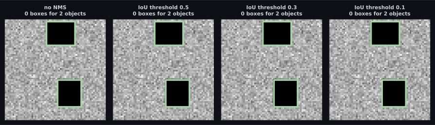

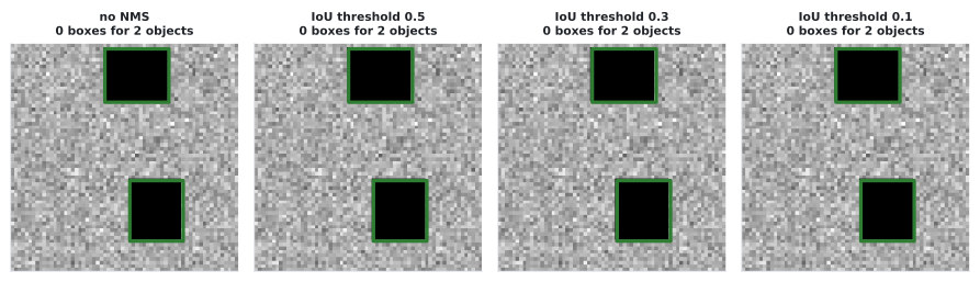
Four panels of the same scene at decreasing NMS IoU thresholds. The leftmost, labelled no NMS, shows several overlapping amber boxes around each object; moving right through thresholds 0.5, 0.3 and 0.1 the duplicates disappear until one box per object remains. — The sort order matters as much as the threshold: NMS is greedy, so the highest-scoring box in each cluster survives and defines what counts as a duplicate. Too high a threshold leaves duplicates; too low deletes genuinely separate objects that happen to overlap — which is why crowded scenes need a higher threshold than sparse ones.

NMS is post-processing: no parameters, no gradients. It cannot improve a box, only remove one, which is why it barely moved precision or recall in the table above — the duplicates it deleted were already matching the same true box.

sketch Non-max suppression, by hand p5.js

Drag the IoU threshold. Boxes are taken in score order; each survives only if it overlaps every survivor by less than the threshold.

Two-stage, one-stage, and what the names mean

Family	Idea	Trade
R-CNN → Fast → Faster	propose regions, then classify each	accurate, slow; Faster R-CNN learns the proposals
YOLO / SSD	one pass, a grid of predictions	one forward pass per image, weaker on small and crowded objects
RetinaNet	one-stage plus focal loss	attacks the negative-majority problem directly
DETR	transformer, set prediction	no anchors, no NMS; needs far longer training

The detector on this page is the YOLO shape reduced to essentials: one grid, one box per cell, one class. Everything a production detector adds — anchors, feature pyramids for multiple scales, focal loss, per-box class heads — answers a limitation you can already measure here.

sketch The measured table, ranked p5.js

Click a column to rank every row by it. The bars are that column's values and the highest and lowest are computed from the numbers, not written in.

Pitfalls

Scoring geometry where there is no object. Measured 38.50× loss inflation on a 2×2 example; at 0.0305 positive cells the real figure is worse.
Forgetting that one cell holds one object. 3.00% of these scenes lose an object to a cell collision, and no amount of training recovers it.
Regressing raw pixel coordinates. Cell-relative offsets and image-relative sizes keep every target in $[0, 1]$ , where a sigmoid lives.
Quoting precision without recall. Precision sat at 0.997 while recall fell 0.8616 → 0.6799: it reported nothing about the threshold change.
Quoting a detection score without its IoU threshold. Exercise 5 shows the same three predictions scoring recall 1.0000 at IoU 0.5 and 0.0000 at 0.75.
Expecting NMS to improve accuracy. It removes duplicates; it cannot make a bad box good, and too low a threshold deletes real neighbouring objects.
Ignoring the objectness bias. Trained against a 32.8:1 negative majority, the head defaults to “nothing here” — which is why the first test scene got zero detections.

Recap

Detection needs a variable-length answer, so a single-stage detector fixes the shape with a grid: 8×8 cells × 5 numbers = 320 outputs, exactly invertible.
Cell-relative offsets and image-relative sizes put every target in $[0, 1]$ .
Only 0.0305 of cells hold an object centre — a 32.8:1 imbalance that forces the masked geometry loss (38.50× inflation without it) and the 5.0 weight with it.
IoU is unforgiving: a 4-pixel shift on a 20-pixel box scores 0.6667, and touching boxes score exactly 0.
Measured at IoU 0.5: recall 0.8616 / 0.7726 / 0.6799 at objectness 0.3 / 0.5 / 0.7, precision flat at ~0.997. The failure mode is misses, not false alarms.
NMS is greedy, parameterless post-processing — 134 duplicates removed at threshold 0.3, 28 at 0.7.

Convolutions carried this entire phase. The last page replaces them with attention and measures what that costs: Vision Transformers (ViT).

pch.quizTag pch.quizDefaultTitle

Why does a detector predict box centres as offsets inside a grid cell rather than as pixel coordinates?

pch.quizShowAnswer

B — So every target lies in [0, 1] and a sigmoid can produce it — a raw-pixel target forces the network to learn the image size as well as the object — The same reasoning applies to width and height, which are scaled by the image side rather than the cell.
Only 0.0305 of cells contain an object centre. What does that force in the loss?

pch.quizShowAnswer

B — Masking the geometry terms by objectness — geometry in an empty cell describes no box, and counting it inflated the geometry loss 38.50x in the worked example — Objectness itself must still be scored in every cell: the model has to learn where objects are not.
Raising the objectness threshold from 0.3 to 0.7 moved recall from 0.8616 to 0.6799 while precision stayed near 0.997. What is the right reading?

pch.quizShowAnswer

B — This detector's errors are misses, not false alarms — so raising the threshold buys almost no precision and costs a great deal of recall — It is the expected shape for a head trained against a 32.8:1 negative majority, and precisely what focal loss addresses.
Two boxes share only an edge — they touch but do not overlap. What is their IoU?

pch.quizShowAnswer

B — Exactly 0 — the intersection has zero area, and IoU has no notion of 'nearly overlapping' — The measured table shows touching boxes and boxes 30 pixels apart both scoring 0.0000.
What is the hard limit of one-box-per-cell, and how do real detectors work around it?

pch.quizShowAnswer

B — Two object centres in the same cell cannot both be represented — measured at 3.00% of scenes here; anchors (several boxes per cell) and finer grids raise the ceiling — It is a representational limit, not an optimisation one — no loss function or training budget can recover the second object.

🧪 Try It Yourself

pch.coffeeTagline

pch.coffeeCta

pch.feedbackHeading

pch.feedbackSubheading

Object Detection (Bounding Boxes and YOLO)

What you’ll learn

IoU first, because everything is scored with it

The grid encoding

The design’s built-in limit

The imbalance, and the loss it forces

What the trained detector does

Non-max suppression

Two-stage, one-stage, and what the names mean

Pitfalls

Recap

Next

🧪 Try It Yourself

pch.feedbackHeading