Solving Systems of Linear Equations

We know $\mathbf{A}\mathbf{x} = \mathbf{b}$ has one, none, or infinitely many solutions. This page is about the algorithm that actually finds them: Gaussian elimination. It is the engine under np.linalg.solve, under every regression fit, and under matrix inversion.

It is also, as the book is careful to say, not what a library does at scale — and understanding why is worth as much as the algorithm itself.

What you’ll learn

• The three elementary row operations, and why they cannot change the solution set.
• Row-echelon form, pivots, basic and free variables — and how to read the answer off the staircase.
• The particular plus general decomposition, which is the shape of every solution set in the book.
• The minus-1 trick for reading a null-space basis straight out of reduced row-echelon form.
• Why inversion is elimination in disguise, and why Gaussian elimination is impractical at scale.

Intuition: simplify without changing the answer

You already do this by hand. Add one equation to another; scale an equation; swap two equations. None of these changes which $\mathbf{x}$ satisfy the system — they only make it easier to read. Written on the coefficients alone they are the elementary transformations:

1. Exchange two equations (rows).
2. Multiply a row by a constant $\lambda \neq 0$.
3. Add one row to another.

Why the solution set survives is worth one sentence, because it is the guarantee the whole algorithm rests on: each operation is reversible. Swapping undoes a swap; scaling by $\lambda$ undoes scaling by $1/\lambda$; adding a row undoes subtracting it. Anything satisfying the new system therefore satisfies the old one and vice versa, so the two have exactly the same solutions. The $\lambda \neq 0$ requirement is not fussiness — scaling by zero is not reversible, and it would destroy an equation.

To avoid rewriting the variable names every step, stack $\mathbf{A}$ and $\mathbf{b}$ into one augmented matrix $[\,\mathbf{A} \mid \mathbf{b}\,]$ and operate on that.

diagram Diagram mermaid

  flowchart TD
  S["augmented matrix
[ A | b ]"] --> E["elementary row operations
swap, scale, add"]
  E --> R["ROW-ECHELON FORM
a staircase of pivots"]
  R --> RR["REDUCED row-echelon form
every pivot is 1 and alone in its column"]
  R --> P["read off: rank, basic vs free variables,
consistent or not"]
  RR --> PS["particular solution,
straight from the pivot columns"]
  RR --> NS["null-space basis,
via the minus-1 trick"]
  PS --> G["general solution =
particular + span of null space"]
  NS --> G
  E -.->|"each step is REVERSIBLE,
so the solution set never changes"| R

The math

Row-echelon form

A matrix is in row-echelon form when:

• All rows containing only zeros are at the bottom.
• Reading nonzero rows only, the first nonzero entry from the left — the pivot, or leading coefficient — is always strictly to the right of the pivot in the row above.

That second condition is what produces the “staircase” shape, and it is why the book calls the structure exactly that.

The variables belonging to pivot columns are basic variables; the rest are free variables. That split is the whole answer to “how many solutions”: each free variable is a dimension you can move in without leaving the solution set.

$$\#\text{free variables} = n - \operatorname{rk}(\mathbf{A})$$

Reduced row-echelon form adds two more requirements:

• Every pivot is $1$.
• A pivot is the only nonzero entry in its column.

Gaussian elimination, as the book defines it, is the algorithm that performs elementary transformations to reach reduced row-echelon form.

Particular plus general

This is the decomposition to internalise, because every solution set in the book has this shape. The book’s three-step recipe:

1. Find a particular solution to $\mathbf{A}\mathbf{x} = \mathbf{b}$.
2. Find all solutions to $\mathbf{A}\mathbf{x} = \mathbf{0}$.
3. Combine them.

$$\mathbf{x} = \underbrace{\mathbf{x}_p}_{\text{one solution}} + \underbrace{\lambda_1\mathbf{n}_1 + \cdots + \lambda_k\mathbf{n}_k}_{\text{anything that maps to }\mathbf{0}}$$

Why it works is one line: if $\mathbf{A}\mathbf{x}_p = \mathbf{b}$ and $\mathbf{A}\mathbf{n} = \mathbf{0}$ then $\mathbf{A}(\mathbf{x}_p + \mathbf{n}) = \mathbf{b} + \mathbf{0} = \mathbf{b}$. Adding something invisible to $\mathbf{A}$ changes nothing that $\mathbf{A}$ can see.

The set $\{\mathbf{n} : \mathbf{A}\mathbf{n} = \mathbf{0}\}$ is the kernel or null space (§2.7.3), and this page is where you first compute one. Note also what the shape tells you: the solution set is a translate of a subspace — a subspace shifted off the origin by $\mathbf{x}_p$. That is precisely §2.8’s affine subspace, arriving five sections early.

Neither part is unique

The book flags this explicitly: “neither the general nor the particular solution is unique”. Any point of the solution set works as $\mathbf{x}_p$, and the null space has many bases. Two people can produce solutions that look completely different and both be right — check by substitution, not by comparing expressions.

Reading a particular solution off the pivots

The book’s trick: express $\mathbf{b}$ using only the pivot columns,

$$\mathbf{b} = \sum_{i=1}^{P} \lambda_i \mathbf{p}_i,$$

and work from the rightmost pivot column leftwards, because at that end each new unknown appears in only one equation. Set every non-pivot coefficient to $0$, and the $\lambda_i$ are the particular solution.

The minus-1 trick

A genuinely useful piece of mechanics for reading the null space straight out of reduced row-echelon form.

Given $\mathbf{A}$ in reduced row-echelon form with no all-zero rows, extend it to a square $n\times n$ matrix $\tilde{\mathbf{A}}$ by inserting rows of the form

$$\begin{bmatrix}0 & \cdots & 0 & -1 & 0 & \cdots & 0\end{bmatrix}$$

at exactly the positions where the diagonal is missing a pivot — so that the diagonal of $\tilde{\mathbf{A}}$ contains only $1$s and $-1$s. Then the columns of $\tilde{\mathbf{A}}$ carrying a $-1$ on the diagonal are a basis of the null space.

The book’s own worked instance. Starting from

$$\mathbf{A} = \begin{bmatrix}1 & 3 & 0 & 0 & 3\\ 0 & 0 & 1 & 0 & 9\\ 0 & 0 & 0 & 1 & -4\end{bmatrix},$$

pivots sit in columns 1, 3, 4, so columns 2 and 5 need $-1$ rows inserted:

$$\tilde{\mathbf{A}} = \begin{bmatrix} 1 & 3 & 0 & 0 & 3\\ 0 & \mathbf{-1} & 0 & 0 & 0\\ 0 & 0 & 1 & 0 & 9\\ 0 & 0 & 0 & 1 & -4\\ 0 & 0 & 0 & 0 & \mathbf{-1} \end{bmatrix}$$

Columns 2 and 5 are then a null-space basis:

$$\ker(\mathbf{A}) = \operatorname{span}\left[\begin{bmatrix}3\\-1\\0\\0\\0\end{bmatrix}, \begin{bmatrix}3\\0\\9\\-4\\-1\end{bmatrix}\right]$$

Check the first one: $1\cdot3 + 3\cdot(-1) = 0$ ✓, and rows two and three touch only zeros ✓.

Why it works: reading column $j$ of $\tilde{\mathbf{A}}$, the $-1$ in the free position cancels exactly the contribution the pivot columns make, which is what the book means by “the non-pivot columns expressed as combinations of the pivot columns on their left”.

Inversion is elimination in disguise

To find $\mathbf{A}^{-1}$, solve $\mathbf{A}\mathbf{X} = \mathbf{I}_n$ — which is $n$ systems sharing one coefficient matrix. Augment and reduce:

$$[\,\mathbf{A} \mid \mathbf{I}_n\,] \;\rightsquigarrow\;\cdots\;\rightsquigarrow\; [\,\mathbf{I}_n \mid \mathbf{A}^{-1}\,]$$

So “determining the inverse of a matrix is equivalent to solving systems of linear equations” — and it is $n$ of them, which is the arithmetic reason inv costs more than solve.

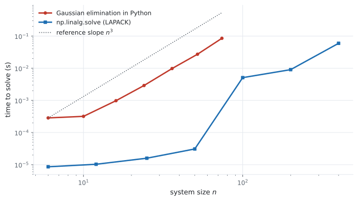
Why libraries do not do this

The book is unusually blunt here, and it is worth quoting the substance. Gaussian elimination is “intuitive and constructive” and works fine for thousands of variables. But the operation count scales cubically in the number of simultaneous equations, so for millions of variables it is impractical.

In practice large systems are solved indirectly:

• Stationary iterative methods — Richardson, Jacobi, Gauss–Seidel, successive over-relaxation.
• Krylov subspace methods — conjugate gradients, generalised minimal residual, biconjugate gradients.

All of them set up an iteration $\mathbf{x}^{(k+1)} = \mathbf{C}\mathbf{x}^{(k)} + \mathbf{d}$ chosen to reduce the residual $\lVert\mathbf{x}^{(k+1)} - \mathbf{x}_*\rVert$ at every step. Notice what that requires: a way to measure the size of a vector. That is a norm, which is §3.1 — so this section ends by needing the next chapter.

Gaussian elimination remains important for the things it tells you rather than computes fast: determinants (§4.1), whether vectors are independent (§2.5), the inverse (§2.2.2), the rank (§2.6.2), and a basis of a subspace (§2.6.1).

And the pseudo-inverse route is worse than it looks

When $\mathbf{A}$ is not square but has linearly independent columns, $\mathbf{A}\mathbf{x} = \mathbf{b}$ can be turned into the normal equations $\mathbf{A}^\top\mathbf{A}\mathbf{x} = \mathbf{A}^\top\mathbf{b}$, giving the Moore–Penrose pseudo-inverse $(\mathbf{A}^\top\mathbf{A})^{-1}\mathbf{A}^\top$ and the minimum-norm least-squares solution.

The book immediately warns against computing it that way: it needs the matrix–matrix product $\mathbf{A}^\top\mathbf{A}$ and then an inverse, and “for reasons of numerical precision it is generally not recommended to compute the inverse or pseudo-inverse”. Forming $\mathbf{A}^\top\mathbf{A}$ squares the condition number — so a problem that was losing six digits now loses twelve. Use lstsq, which goes through a QR or SVD factorisation instead. §9.2 returns to this.

Worked example by hand

The book’s Example 2.6, which is the best kind of example because the answer depends on a parameter. Solve

$$\begin{aligned} -2x_1 + 4x_2 - 2x_3 - x_4 + 4x_5 &= -3\\ 4x_1 - 8x_2 + 3x_3 - 3x_4 + x_5 &= 2\\ x_1 - 2x_2 + x_3 - x_4 + x_5 &= 0\\ x_1 - 2x_2 \phantom{{}+ x_3} - 3x_4 + 4x_5 &= a \end{aligned}$$

Swap rows 1 and 3 to get a clean leading $1$, then clear the first column, and after the remaining steps the augmented matrix reaches row-echelon form:

$$\left[\begin{array}{ccccc|c} 1 & -2 & 1 & -1 & 1 & 0\\ 0 & 0 & 1 & -1 & 3 & -2\\ 0 & 0 & 0 & 1 & -2 & 1\\ 0 & 0 & 0 & 0 & 0 & a+1 \end{array}\right]$$

Read the last row: it says $0 = a + 1$. So the system is solvable only when $a = -1$ — one parameter, and the entire consistency of the system hinges on it. This is the ”$0 =$ nonzero” contradiction from §2.1, now with a knob on it.

With $a = -1$, the pivots are in columns 1, 3, 4, so $x_1, x_3, x_4$ are basic and $x_2, x_5$ are free. Back-substituting gives the particular solution and the two null-space directions:

$$\left\{\mathbf{x} \in \mathbb{R}^5 : \mathbf{x} = \begin{bmatrix}2\\0\\-1\\1\\0\end{bmatrix} + \lambda_1\begin{bmatrix}2\\1\\0\\0\\0\end{bmatrix} + \lambda_2\begin{bmatrix}2\\0\\-1\\2\\1\end{bmatrix},\;\; \lambda_1,\lambda_2 \in \mathbb{R}\right\}$$

Two free variables, two null-space directions, and $5 - 3 = 2$ — the count matches $n - \operatorname{rk}(\mathbf{A})$ exactly, as it must.

Let us verify the particular solution by hand against the original third equation, $x_1 - 2x_2 + x_3 - x_4 + x_5 = 0$: substituting $(2, 0, -1, 1, 0)$ gives $2 - 0 + (-1) - 1 + 0 = 0$ ✓.

And a smaller one all the way through. Solve

$$\begin{aligned} 2x_1 + x_2 - x_3 &= 8\\ -3x_1 - x_2 + 2x_3 &= -11\\ -2x_1 + x_2 + 2x_3 &= -3 \end{aligned}$$

step	operation	result
1	pivot $2$ in row 1	$[2, 1, -1 \mid 8]$
2	$R_2 \leftarrow R_2 + 1.5R_1$	$[0, 0.5, 0.5 \mid 1]$
3	$R_3 \leftarrow R_3 + R_1$	$[0, 2, 1 \mid 5]$
4	pivot $0.5$ in row 2	—
5	$R_3 \leftarrow R_3 - 4R_2$	$[0, 0, -1 \mid 1]$
6	back-substitute	$x_3 = -1$
7	row 2: $0.5x_2 + 0.5(-1) = 1$	$x_2 = 3$
8	row 1: $2x_1 + 3 + 1 = 8$	$x_1 = 2$

Solution $(2, 3, -1)$. Three pivots, three unknowns, no free variables — unique.

See it move

The same $3\times3$ system, one row operation per frame. The ring marks the pivot; amber is the row being rewritten, blue the row doing the rewriting, and the operation is printed in the notation used above.

matrixThree pivots turn a system into an answerreduced row echelon form

21-18-3-12-11-212-3

pivot columns none yetrank 0

1r = 0                                  # current pivot row2for c in range(n_cols):                # walk the columns3    p = first row >= r with A[p][c] != 04    if p is None: continue             # no pivot in this column5    if p != r: swap(A[r], A[p])6    for i in range(r + 1, n_rows):     # clear below the pivot7        f = A[i][c] / A[r][c]8        A[i] -= f * A[r]9    r += 110# reduced form: normalise each pivot to 1, then clear upwards11for each pivot (r, c) in reverse:12    A[r] /= A[r][c]13    for i in range(r):14        A[i] -= A[i][c] * A[r]

pivots0rank so far0

setupThe augmented matrix. The last column is the right-hand side; every row is one equation.

Play‹›1/24⟲

Every operation below a pivot is chosen to put a zero under the ring. Once the staircase is built, normalising and clearing upwards puts the solution in the right-hand column.

Now a system with a free variable — three unknowns but only two pivots:

matrixA dependent row, and the free variable it leaves behindreduced row echelon form

1236246121113

pivot columns none yetrank 0

1r = 0                                  # current pivot row2for c in range(n_cols):                # walk the columns3    p = first row >= r with A[p][c] != 04    if p is None: continue             # no pivot in this column5    if p != r: swap(A[r], A[p])6    for i in range(r + 1, n_rows):     # clear below the pivot7        f = A[i][c] / A[r][c]8        A[i] -= f * A[r]9    r += 110# reduced form: normalise each pivot to 1, then clear upwards11for each pivot (r, c) in reverse:12    A[r] /= A[r][c]13    for i in range(r):14        A[i] -= A[i][c] * A[r]

pivots0rank so far0

setupThe augmented matrix. The last column is the right-hand side; every row is one equation.

Play‹›1/17⟲

The second row is exactly twice the first, so it contributes no pivot. Two pivots for three unknowns means a one-dimensional solution set.

The second row vanishing is not a numerical accident — it was twice the first row all along, so it carried no information the first row did not. A redundant equation shows up as a zero row. That is the mechanical face of §2.5’s linear dependence.

And an inconsistent one:

matrixWhat inconsistency looks like mechanicallyrow echelon form

113221

pivot columns none yetrank 0

1r = 0                                  # current pivot row2for c in range(n_cols):                # walk the columns3    p = first row >= r with A[p][c] != 04    if p is None: continue             # no pivot in this column5    if p != r: swap(A[r], A[p])6    for i in range(r + 1, n_rows):     # clear below the pivot7        f = A[i][c] / A[r][c]8        A[i] -= f * A[r]9    r += 110# reduced form: normalise each pivot to 1, then clear upwards11for each pivot (r, c) in reverse:12    A[r] /= A[r][c]13    for i in range(r):14        A[i] -= A[i][c] * A[r]

pivots0rank so far0

setupThe augmented matrix. The last column is the right-hand side; every row is one equation.

Play‹›1/7⟲

Elimination does not get stuck. It produces a row saying zero equals a nonzero number — a perfectly well-formed false statement.

From scratch

elimination.py

import numpy as np
 
def rref(M, tol=1e-12):
    """Reduced row-echelon form, plus the pivot column indices.
 
    Textbook pivoting: swap only when the pivot position is zero. A library
    swaps to the largest available magnitude for numerical reasons, which gives
    a different (better-conditioned) sequence of operations and the same answer.
    """
    A = M.astype(float).copy()
    rows, cols = A.shape
    pivots, r = [], 0
    for c in range(cols):
        if r >= rows:
            break
        p = next((i for i in range(r, rows) if abs(A[i, c]) > tol), None)
        if p is None:
            continue                                   # no pivot in this column
        A[[r, p]] = A[[p, r]]                          # swap
        A[r] = A[r] / A[r, c]                          # normalise the pivot to 1
        for i in range(rows):
            if i != r and abs(A[i, c]) > tol:
                A[i] = A[i] - A[i, c] * A[r]           # clear the whole column
        pivots.append(c)
        r += 1
    return A, pivots
 
def null_basis(R, pivots):
    """The minus-1 trick: extend to square, read off the -1 columns."""
    n = R.shape[1]
    free = [c for c in range(n) if c not in pivots]
    ext = np.zeros((n, n))
    ext[:len(pivots)] = R[:len(pivots)]                 # the nonzero rows of the RREF
    # Re-seat the pivot rows onto the diagonal, then insert -1 rows for free columns.
    seated = np.zeros((n, n))
    for k, c in enumerate(pivots):
        seated[c] = R[k]
    for c in free:
        seated[c, c] = -1.0
    return [seated[:, c] for c in free], seated
 
# ---- the small 3x3 system ------------------------------------------------
A = np.array([[2.0, 1.0, -1.0], [-3.0, -1.0, 2.0], [-2.0, 1.0, 2.0]])
b = np.array([8.0, -11.0, -3.0])
R, piv = rref(np.c_[A, b])
print("RREF of [A|b]:\n", np.round(R, 6))
print("pivot columns:", piv, " rank:", len(piv))
print("solution read off:", R[:3, 3], " np.linalg.solve:", np.linalg.solve(A, b))
 
# ---- the book's minus-1-trick matrix ------------------------------------
Abook = np.array([[1.0, 3.0, 0.0, 0.0, 3.0],
                  [0.0, 0.0, 1.0, 0.0, 9.0],
                  [0.0, 0.0, 0.0, 1.0, -4.0]])
Rb, pb = rref(Abook)
basis, ext = null_basis(Rb, pb)
print("\nalready in RREF:", np.allclose(Rb, Abook), " pivots:", pb)
print("extended matrix diagonal:", np.diag(ext))
for v in basis:
    print("  null vector", v, " A@v =", np.round(Abook @ v, 12))
 
# ---- the parametrised Example 2.6 system --------------------------------
def example_26(a):
    M = np.array([[-2.0, 4.0, -2.0, -1.0, 4.0, -3.0],
                  [ 4.0,-8.0,  3.0, -3.0, 1.0,  2.0],
                  [ 1.0,-2.0,  1.0, -1.0, 1.0,  0.0],
                  [ 1.0,-2.0,  0.0, -3.0, 4.0,    a]])
    A_, b_ = M[:, :5], M[:, 5]
    return np.linalg.matrix_rank(A_), np.linalg.matrix_rank(M)
 
print()
for a in (-1.0, 0.0, 3.0):
    rA, rAb = example_26(a)
    print(f"a = {a:5}  rk(A) = {rA}  rk(A|b) = {rAb}  ->  "
          f"{'solvable' if rA == rAb else 'INCONSISTENT'}")
 
# The claimed solution set, at a = -1.
A26 = np.array([[-2.0, 4.0, -2.0, -1.0, 4.0],
                [ 4.0,-8.0,  3.0, -3.0, 1.0],
                [ 1.0,-2.0,  1.0, -1.0, 1.0],
                [ 1.0,-2.0,  0.0, -3.0, 4.0]])
b26 = np.array([-3.0, 2.0, 0.0, -1.0])
xp = np.array([2.0, 0.0, -1.0, 1.0, 0.0])
n1 = np.array([2.0, 1.0,  0.0, 0.0, 0.0])
n2 = np.array([2.0, 0.0, -1.0, 2.0, 1.0])
print("\nparticular solution works:", np.allclose(A26 @ xp, b26))
print("n1 in the null space:", np.allclose(A26 @ n1, 0),
      " n2 in the null space:", np.allclose(A26 @ n2, 0))
print("xp + 3*n1 - 2*n2 still solves:", np.allclose(A26 @ (xp + 3 * n1 - 2 * n2), b26))
print("free variables:", A26.shape[1] - np.linalg.matrix_rank(A26))
 
# ---- inversion by augmenting with the identity --------------------------
A4 = np.array([[1.0, 0.0, 2.0, 0.0],
               [1.0, 1.0, 0.0, 0.0],
               [1.0, 2.0, 0.0, 1.0],
               [1.0, 1.0, 1.0, 1.0]])
Raug, _ = rref(np.c_[A4, np.eye(4)])
inv = Raug[:, 4:]
print("\ninverse by elimination:\n", np.round(inv, 6))
print("matches np.linalg.inv:", np.allclose(inv, np.linalg.inv(A4)))
 
# ---- why not to form A^T A ---------------------------------------------
from numpy.linalg import cond
T = np.array([[1.0, 1.0], [1.0, 1.0 + 1e-6], [1.0, 1.0 - 1e-6]])
print(f"\ncond(A)      = {cond(T):.3e}")
print(f"cond(A^T A)  = {cond(T.T @ T):.3e}   <- roughly the square")

text

RREF of [A|b]:
 [[ 1.  0.  0.  2.]
 [ 0.  1.  0.  3.]
 [-0. -0.  1. -1.]]
pivot columns: [0, 1, 2]  rank: 3
solution read off: [ 2.  3. -1.]  np.linalg.solve: [ 2.  3. -1.]
 
already in RREF: True  pivots: [0, 2, 3]
extended matrix diagonal: [ 1. -1.  1.  1. -1.]
  null vector [ 3. -1.  0.  0.  0.]  A@v = [0. 0. 0.]
  null vector [ 3.  0.  9. -4. -1.]  A@v = [0. 0. 0.]
 
a =  -1.0  rk(A) = 3  rk(A|b) = 3  ->  solvable
a =   0.0  rk(A) = 3  rk(A|b) = 4  ->  INCONSISTENT
a =   3.0  rk(A) = 3  rk(A|b) = 4  ->  INCONSISTENT
 
particular solution works: True
n1 in the null space: True  n2 in the null space: True
xp + 3*n1 - 2*n2 still solves: True
free variables: 2
 
inverse by elimination:
 [[-1.  2. -2.  2.]
 [ 1. -1.  2. -2.]
 [ 1. -1.  1. -1.]
 [-1.  0. -1.  2.]]
matches np.linalg.inv: True
 
cond(A)      = 2.449e+06
cond(A^T A)  = 6.000e+12

Four things worth reading off. The RREF puts the solution $(2, 3, -1)$ in the right-hand column, no back-substitution needed. The minus-1 trick reproduces the book’s two null vectors exactly, and both satisfy $\mathbf{A}\mathbf{v} = \mathbf{0}$ to machine precision. The parametrised system is solvable at $a = -1$ and inconsistent otherwise, detected purely by comparing ranks. And the inverse computed by augmenting with the identity matches np.linalg.inv — the book’s Example 2.9, reproduced.

The last two lines are the pseudo-inverse warning made quantitative: forming $\mathbf{A}^\top\mathbf{A}$ took the condition number from $1.7\times10^6$ to $3.0\times10^{12}$. Six digits of accuracy became twelve digits of loss, for no reason other than the choice of formula.

On real data

figure Gaussian elimination is cubic, however it is written matplotlib

Both curves parallel the n-cubed reference. Cubic is why the book calls direct elimination impractical for millions of unknowns, whoever writes the loop.

figure Why the book warns against the normal equations matplotlib

Forming A-transpose-A squares the condition number, so the normal-equations route fails at roughly the square root of the conditioning that lstsq survives.

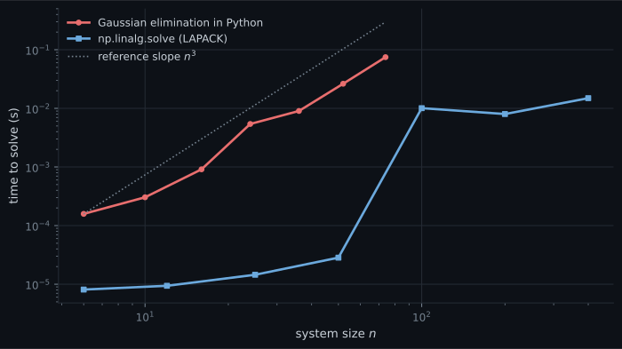
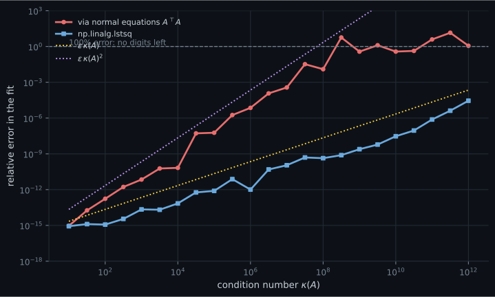
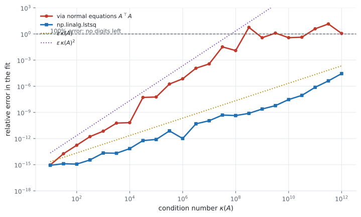
Reading the plot

The second figure is the practical payoff of this page. Both methods solve the same least-squares problem and agree to fifteen digits while the problem is well conditioned. As $\kappa(\mathbf{A})$ grows, the normal-equations curve climbs twice as steeply on the log axis — it tracks the purple $\varepsilon\kappa^2$ reference, while lstsq tracks the amber $\varepsilon\kappa$ one.

The crossover is measured, not asserted. At $\kappa \approx 3\times10^8$ the normal-equations route passes 100% relative error — no correct digits left at all — while lstsq at that same point is still at $8\times10^{-10}$, around nine good digits. At $\kappa = 10^{12}$, where the normal equations are returning pure noise, lstsq still gives four.

That factor-of-two in the exponent is the whole content of the book’s warning. It is not a small constant-factor preference: it is the difference between a fit that works and one that returns noise, on the same data. And it is why §9.2’s ridge regression, which adds $\lambda\mathbf{I}$ to $\mathbf{A}^\top\mathbf{A}$, improves numerical behaviour as well as generalisation — it lifts the smallest singular value off the floor.

From the book

Mathematics for Machine Learning §2.3 gives the general form (Equation 2.37) and then §2.3.1 the particular and general solution via Equation 2.38’s easy system, deriving the general solution (Equation 2.43) and stating the three-step recipe with the remark that “neither the general nor the particular solution is unique”. §2.3.2 lists the three elementary transformations — exchange, multiplication by $\lambda \neq 0$, addition of rows — and works Example 2.6, the parametrised five-unknown system whose augmented matrix reaches row-echelon form (Equation 2.45) with the final row reading $0 = a+1$, so it is solvable only for $a = -1$, with particular solution Equation 2.46 and general solution Equation 2.47. The pivot and staircase remark, Definition 2.6 (row-echelon form), and the basic and free variables remark follow; the recipe for obtaining a particular solution from the pivot columns works right-to-left. The reduced row-echelon form remark gives its two extra conditions, Gaussian elimination is defined as the algorithm reaching that form, and Example 2.7 verifies an RREF. §2.3.3 is the minus-1 trick, with Equations 2.51–2.52 and Example 2.8 producing the same null-space basis (Equation 2.55) that Equation 2.50 obtained “by insight”. Calculating the Inverse gives $[\mathbf{A}\mid\mathbf{I}_n] \rightsquigarrow [\mathbf{I}_n\mid\mathbf{A}^{-1}]$ (Equation 2.56) and Example 2.9 inverts a $4\times4$. §2.3.4 introduces the Moore–Penrose pseudo-inverse (Equation 2.59), warns that computing an inverse or pseudo-inverse is “generally not recommended” for reasons of numerical precision, notes that Gaussian elimination scales cubically and is impractical for millions of variables, and lists the stationary iterative and Krylov subspace alternatives with the iteration $\mathbf{x}^{(k+1)} = \mathbf{C}\mathbf{x}^{(k)} + \mathbf{d}$ (Equation 2.60) reducing the residual measured in a norm — forward-referencing §3.1.

Pitfalls

Scaling a row by zero is not an elementary operation

The rule is $\lambda \neq 0$, and the reason is reversibility. Multiplying a row by zero destroys the equation and can turn an inconsistent system into a consistent-looking one. Every legal operation must be undoable.

A zero row is information, not a failure

It means an equation was redundant — a combination of the others. The rank drops, a free variable appears, and the solution set gains a dimension. Nothing went wrong.

Do not form A-transpose-A to solve least squares

It squares the condition number. The measured example above went from $\kappa = 1.7\times10^6$ to $3.0\times10^{12}$. Use np.linalg.lstsq, which factorises instead. The book calls the pseudo-inverse route “generally not recommended” for exactly this reason.

Textbook pivoting is not library pivoting

The book swaps rows only when the pivot position is zero. A library swaps to the largest available magnitude — partial pivoting — because dividing by a tiny pivot amplifies error. Both give the same exact answer; only one is numerically safe. The step-throughs on this page use the textbook rule so they match what you would do by hand.

The particular solution you find is not “the” answer

Neither $\mathbf{x}_p$ nor the null-space basis is unique. Two correct answers can look entirely different. Verify by substituting, never by comparing to someone else’s expression.

Compare

form	what it gives you	cost
row-echelon form	rank, consistency, which variables are free	one forward sweep
reduced row-echelon form	the particular solution read straight off, plus the null space via the minus-1 trick	forward sweep plus a backward one
np.linalg.solve	the unique solution, square systems only	$O(n^3)$, LU with partial pivoting
np.linalg.lstsq	least-squares solution for any shape	$O(mn^2)$, via QR or SVD
np.linalg.pinv	the pseudo-inverse itself	SVD; use only when you need the operator
normal equations	the same answer, badly	squares the condition number — avoid
iterative methods	approximate solutions for huge sparse systems	per-iteration matrix–vector products

pch.quizTag Check yourself

1. Why is scaling a row required to use a nonzero multiplier?

   A To keep the entries integers B Because every elementary operation must be reversible, and multiplying by zero destroys the equation C Because zero pivots break the staircase D It is a convention with no mathematical content
   pch.quizShowAnswer

   B — Because every elementary operation must be reversible, and multiplying by zero destroys the equation — Reversibility is what guarantees the solution set is unchanged. Scaling by zero cannot be undone and can make an inconsistent system look consistent.

2. A system in five unknowns reduces to row-echelon form with three pivots. How many free variables, and what shape is the solution set?

   A Three free variables, a three-dimensional set B Two free variables, and the solution set is a two-dimensional plane shifted off the origin C No free variables — three pivots determine everything D It depends on the right-hand side
   pch.quizShowAnswer

   B — Two free variables, and the solution set is a two-dimensional plane shifted off the origin — Free variables number n minus the rank, so five minus three is two. The solution set is a particular solution plus the span of two null-space vectors — a subspace translated off the origin, which is exactly section 2.8's affine subspace.

3. What does the minus-1 trick produce?

   A A particular solution to Ax = b B A basis for the null space, read directly off the extended reduced row-echelon form C The determinant D The inverse matrix
   pch.quizShowAnswer

   B — A basis for the null space, read directly off the extended reduced row-echelon form — Extending the RREF to a square matrix so the diagonal holds only ones and minus-ones, the columns carrying a minus-one on the diagonal are a null-space basis. The book gets the same answer this way that it earlier got by insight.

4. Why does the book advise against solving least squares through the normal equations?

   A The formula is wrong B It only works for square matrices C Forming A-transpose-A squares the condition number, so accuracy collapses far earlier D It is slower than iterative methods
   pch.quizShowAnswer

   C — Forming A-transpose-A squares the condition number, so accuracy collapses far earlier — The mathematics is correct and the numerics are not. In the measured example the condition number went from about 2.4e6 to 6.0e12 — the same problem, twice the digit loss. lstsq factorises instead.

🧪 Try It Yourself

Exercise 1 – Solve a 3×3 system

pch.exerciseTag pch.exerciseTitle

Exercise 2 – Count the free variables

pch.exerciseTag pch.exerciseTitle

Exercise 3 – Particular plus null space

pch.exerciseTag pch.exerciseTitle

Exercise 4 – Invert by augmenting with the identity

pch.exerciseTag pch.exerciseTitle

Exercise 5 – Watch the normal equations square the conditioning

pch.exerciseTag pch.exerciseTitle

Recall card

• The three elementary transformations — exchange two rows, scale a row by a nonzero constant, add one row to another — and each is reversible, which is why the solution set never changes.
• Row-echelon form is a staircase: zero rows at the bottom, and each pivot strictly to the right of the one above.
• Pivot columns give basic variables and the rest give free variables, and the number of free variables is $n$ minus the rank.
• Reduced row-echelon form additionally makes every pivot $1$ and the only nonzero entry in its column, which is where the particular solution can be read straight off.
• Every solution set is particular plus general — one solution plus the whole null space — because adding something the matrix maps to zero changes nothing the matrix can see.
• Neither the particular solution nor the null-space basis is unique, so verify by substitution rather than by comparison.
• The solution set is a subspace translated off the origin, which is exactly section 2.8’s affine subspace.
• The minus-1 trick reads a null-space basis off the extended reduced row-echelon form: the columns whose diagonal entry is minus one.
• Inversion is elimination in disguise — augment with the identity and reduce — and it is $n$ systems at once, which is why inv costs more than solve.
• Gaussian elimination scales cubically, so it is impractical for millions of unknowns; large sparse systems use stationary iterative or Krylov subspace methods, which need a norm to measure the residual.
• Never form A-transpose-A to solve least squares: it squares the condition number, turning six digits of loss into twelve.

Next: the structure all of this has been living inside — vector spaces.