What you’ll learn

• the four group fairness criteria, defined precisely, computed on the same model
• why a model that never sees the protected attribute still produces a 0.6537 selection-rate gap
• Chouldechova’s identity, verified to four decimals: prevalence, precision and error rates are algebraically locked together
• why demographic parity, equal opportunity and predictive parity cannot all hold when base rates differ — and what each one costs when you force it
• how to write a bias audit that survives contact with a real dataset
• why “we removed the protected attribute” is not a defence

A deliberately clean setup

Every ingredient here is honest. There is one feature qq — read it as a genuine, unbiased qualification score. It is equally predictive in both groups. The label is generated from qq alone, by the same rule for everybody:

rng = np.random.default_rng(7)
n = 8000
 
group = rng.integers(0, 2, n)
q = rng.normal(np.where(group == 1, -1.1, 1.1), 1.0, n)      # the ONLY difference
y = (rng.random(n) < 1 / (1 + np.exp(-1.6 * q))).astype(int)  # same rule for both
 
X = pd.DataFrame({"q": q, "noise": rng.normal(0, 1, n)})      # note: no `group` column

rng = np.random.default_rng(7)
n = 8000
 
group = rng.integers(0, 2, n)
q = rng.normal(np.where(group == 1, -1.1, 1.1), 1.0, n)      # the ONLY difference
y = (rng.random(n) < 1 / (1 + np.exp(-1.6 * q))).astype(int)  # same rule for both
 
X = pd.DataFrame({"q": q, "noise": rng.normal(0, 1, n)})      # note: no `group` column

Read the third line carefully. $P(y \mid q)$ is identical across groups. The groups differ only in the distribution of $q$ itself — one has, on average, a lower qualification score, for reasons outside the model’s data. That is the entire source of everything that follows.

And note the fourth line: groupgroup is not a feature. The model never sees it.

model = RandomForestClassifier(n_estimators=400, random_state=0).fit(X_train, y_train)
proba = model.predict_proba(X_test)[:, 1]
 
print(f"{model.score(X_test, y_test):.4f}")             # 0.8000
for g in (0, 1):                                        # ranking quality per group
    m = group_test == g
    print(f"group {g} AUC {roc_auc_score(y_test[m], proba[m]):.4f}")
# group 0 AUC 0.7888
# group 1 AUC 0.8042

model = RandomForestClassifier(n_estimators=400, random_state=0).fit(X_train, y_train)
proba = model.predict_proba(X_test)[:, 1]
 
print(f"{model.score(X_test, y_test):.4f}")             # 0.8000
for g in (0, 1):                                        # ranking quality per group
    m = group_test == g
    print(f"group {g} AUC {roc_auc_score(y_test[m], proba[m]):.4f}")
# group 0 AUC 0.7888
# group 1 AUC 0.8042

Accuracy 0.8000. AUC 0.7888 and 0.8042 — the model ranks candidates about equally well inside both groups, and if anything slightly better in group 1. By every conventional check this model is fine.

The four criteria

Fix a threshold $t$, let $\hat{y} = \mathbb{1}[\,\hat{p} \ge t\,]$, and let $A$ be the group.

These are not variations on a theme. They are different demands, and the next section shows they are mutually exclusive here.

What the base rates do

figureBase rates 0.7524 and 0.2147 — model accuracy 0.8000, no measurement bias anywherematplotlib

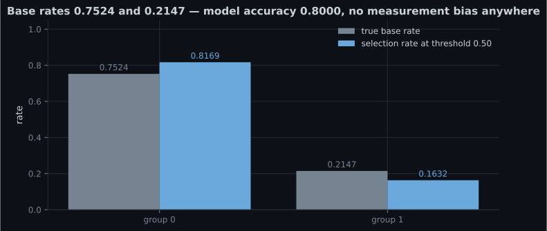
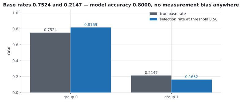
At a single threshold of 0.50, applied identically to everyone:

Three points deserve attention.

The gaps are large and the model is not broken. 0.6537 is not a rounding artefact; it is what “one threshold for everyone” produces when the underlying rates are 0.7524 and 0.2147.

Removing the protected attribute achieved nothing. groupgroup was never a column. qq carries the group difference perfectly well on its own, and any sufficiently rich feature set will. “Fairness through unawareness” is not a technique; it is a way of not looking.

The direction of unfairness depends on which criterion you invoke. Group 1 is selected far less often (bad by demographic parity) and has a much lower false positive rate (good, if a positive is a punishment). Nothing about the numbers alone tells you which reading is right.

The gaps are locked together algebraically

The reason you cannot fix all of these at once is not statistical, it is arithmetic. For any classifier and any group, with prevalence $p$, precision (PPV) and false negative rate $\mathrm{FNR} = 1 - \mathrm{TPR}$:

This is Chouldechova’s identity. It is a rearrangement of the confusion matrix, so it holds exactly, always. Verify it on both groups:

for row in group_rows:
    p = y_test[group_test == row["group"]].mean()
    ppv, fnr = row["precision"], 1 - row["tpr"]
    implied = (p / (1 - p)) * ((1 - ppv) / ppv) * (1 - fnr)
    print(f"group {row['group']}  prevalence {p:.4f}  "
          f"implied FPR {implied:.4f}  measured FPR {row['fpr']:.4f}")
 
# group 0  prevalence 0.7524  implied FPR 0.5430  measured FPR 0.5430
# group 1  prevalence 0.2147  implied FPR 0.0925  measured FPR 0.0925

for row in group_rows:
    p = y_test[group_test == row["group"]].mean()
    ppv, fnr = row["precision"], 1 - row["tpr"]
    implied = (p / (1 - p)) * ((1 - ppv) / ppv) * (1 - fnr)
    print(f"group {row['group']}  prevalence {p:.4f}  "
          f"implied FPR {implied:.4f}  measured FPR {row['fpr']:.4f}")
 
# group 0  prevalence 0.7524  implied FPR 0.5430  measured FPR 0.5430
# group 1  prevalence 0.2147  implied FPR 0.0925  measured FPR 0.0925

Exact to four decimals in both groups, because it is an identity and not an approximation.

Now read it as a constraint. Suppose you equalise PPV across groups (predictive parity) and also equalise FNR (part of equalized odds). Then everything on the right-hand side is equal across groups except $p/(1-p)$ — so FPR must differ, in the ratio of the prevalence odds. Here those odds are 3.0393 and 0.2733, a ratio of 11.1. There is no classifier, no architecture, no amount of data that escapes this. When base rates differ, predictive parity and equalized odds are incompatible except in the degenerate case of a perfect classifier.

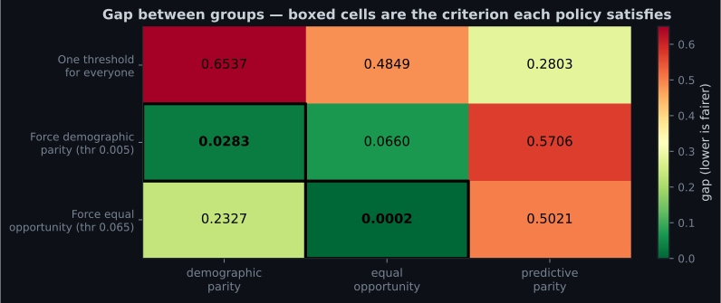
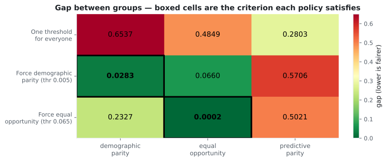
Three policies, three different failures

Take the same model and only change the thresholds. Solve for the group-1 threshold that equalises each criterion in turn:

figureGap between groups — boxed cells are the criterion each policy satisfiesmatplotlib

Look at the thresholds. To reach demographic parity, group 1’s threshold falls to 0.0050 — the model must approve essentially anyone whose predicted probability is not zero. That is what closing a 0.6537 gap by threshold surgery actually requires, and the accuracy cost is 0.7994 → 0.6103.

Interestingly, the last row shows that equalized odds is nearly reachable: at a threshold of 0.0450 the FPR gap is 0.0012 and the TPR gap 0.0181 (the bisection lands group 1’s FPR at 0.5442 against group 0’s 0.5430, since probabilities come in discrete steps). Both error rates roughly matched — and the precision gap has grown to 0.5182. The identity is not negotiable.

Who pays for parity

figureGroup 1 under parity: more selected and more true positives, but precision collapsesmatplotlib

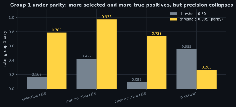
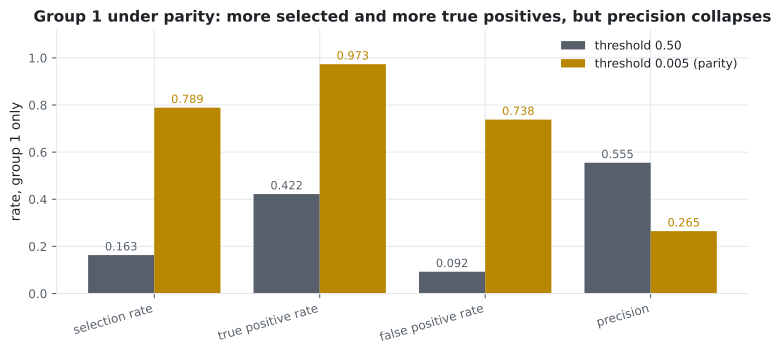
This is the part that gets skipped. Forcing demographic parity does real good — the TPR for group 1 goes from 0.4222 to 0.9731, meaning most of the qualified people who were previously refused now succeed. It also means 73.81% of unqualified group-1 applicants are now approved, against 54.30% in group 0, and that a group-1 approval carries 0.2649 precision against group 0’s 0.8354.

Whether that trade is right depends entirely on what the decision does to people:

There is no default. Picking one of these rows is the fairness work; computing the metric afterwards is the easy part.

See it move

Threshold changes are the only lever most teams actually have, so it is worth developing intuition for what they can and cannot do. Below, two groups have the same score distributions conditional on the label — positives around $+1$, negatives around $-1$ — and differ only in base rate: 0.75 against 0.25. Everything is computed in closed form from the normal CDF, so nothing is approximated except $\Phi$ itself:

Drag the two threshold handles and try to make all three gaps small at once.

Two gaps can be closed at once only in the limit where you select everybody or nobody. The third never cooperates, and that is the impossibility result rendered as a toy.

Writing an audit that is actually useful

A fairness audit is not a single number. It is a table, sliced by group, with counts attached so you can tell a real gap from four unlucky rows.

"""A group fairness report. No dependencies beyond numpy."""
 
import numpy as np
 
 
def group_report(proba, y_true, group, thresholds=None, default_threshold=0.5,
                 min_count=100):
    """Per-group rates at a threshold, plus the gaps and a small-sample warning.
 
    `thresholds` maps group -> threshold, so you can audit a policy that treats
    groups differently as easily as one that does not.
    """
    rows = []
    for g in sorted(set(group)):
        mask = group == g
        t = default_threshold if thresholds is None else thresholds[g]
        pred = (proba[mask] >= t).astype(int)
        yy = y_true[mask]
        positives, selected = yy == 1, pred == 1
        rows.append({
            "group": g,
            "n": int(mask.sum()),
            "n_positive": int(positives.sum()),
            "threshold": t,
            "base_rate": float(yy.mean()),
            "selection": float(pred.mean()),
            "tpr": float(pred[positives].mean()) if positives.any() else np.nan,
            "fpr": float(pred[~positives].mean()) if (~positives).any() else np.nan,
            "precision": float(yy[selected].mean()) if selected.any() else np.nan,
        })
 
    header = f"{'group':>7s} {'n':>6s} {'base':>7s} {'sel':>7s} {'tpr':>7s} {'fpr':>7s} {'prec':>7s}"
    print(header)
    for r in rows:
        warn = "  (n too small to trust)" if r["n"] < min_count else ""
        print(f"{r['group']!s:>7s} {r['n']:6d} {r['base_rate']:7.4f} "
              f"{r['selection']:7.4f} {r['tpr']:7.4f} {r['fpr']:7.4f} "
              f"{r['precision']:7.4f}{warn}")
 
    def spread(key):
        values = [r[key] for r in rows if not np.isnan(r[key])]
        return max(values) - min(values)
 
    print(f"\ndemographic parity gap {spread('selection'):.4f}")
    print(f"equal opportunity gap  {spread('tpr'):.4f}")
    print(f"equal FPR gap          {spread('fpr'):.4f}")
    print(f"predictive parity gap  {spread('precision'):.4f}")
    return rows

"""A group fairness report. No dependencies beyond numpy."""
 
import numpy as np
 
 
def group_report(proba, y_true, group, thresholds=None, default_threshold=0.5,
                 min_count=100):
    """Per-group rates at a threshold, plus the gaps and a small-sample warning.
 
    `thresholds` maps group -> threshold, so you can audit a policy that treats
    groups differently as easily as one that does not.
    """
    rows = []
    for g in sorted(set(group)):
        mask = group == g
        t = default_threshold if thresholds is None else thresholds[g]
        pred = (proba[mask] >= t).astype(int)
        yy = y_true[mask]
        positives, selected = yy == 1, pred == 1
        rows.append({
            "group": g,
            "n": int(mask.sum()),
            "n_positive": int(positives.sum()),
            "threshold": t,
            "base_rate": float(yy.mean()),
            "selection": float(pred.mean()),
            "tpr": float(pred[positives].mean()) if positives.any() else np.nan,
            "fpr": float(pred[~positives].mean()) if (~positives).any() else np.nan,
            "precision": float(yy[selected].mean()) if selected.any() else np.nan,
        })
 
    header = f"{'group':>7s} {'n':>6s} {'base':>7s} {'sel':>7s} {'tpr':>7s} {'fpr':>7s} {'prec':>7s}"
    print(header)
    for r in rows:
        warn = "  (n too small to trust)" if r["n"] < min_count else ""
        print(f"{r['group']!s:>7s} {r['n']:6d} {r['base_rate']:7.4f} "
              f"{r['selection']:7.4f} {r['tpr']:7.4f} {r['fpr']:7.4f} "
              f"{r['precision']:7.4f}{warn}")
 
    def spread(key):
        values = [r[key] for r in rows if not np.isnan(r[key])]
        return max(values) - min(values)
 
    print(f"\ndemographic parity gap {spread('selection'):.4f}")
    print(f"equal opportunity gap  {spread('tpr'):.4f}")
    print(f"equal FPR gap          {spread('fpr'):.4f}")
    print(f"predictive parity gap  {spread('precision'):.4f}")
    return rows

Four rules make the difference between an audit and a ritual:

1. Report every criterion, not the one that looks best. A report showing only the criterion your model happens to satisfy is worse than no report, because it implies the others were checked.
2. Print the counts. A 0.30 gap on 40 people is noise; the same gap on 4,000 is a finding. Attach a confidence interval or at least a minimum-count warning.
3. Slice intersectionally, then stop where the counts run out. Gaps often live in the intersections, and the cells get small fast. Say where you stopped and why.
4. Audit the threshold you actually deploy. Metrics at 0.50 are irrelevant if operations uses 0.31.

The audit as a procedure

The order of these steps is load-bearing: the label question comes first, because a criterion chosen before the label is examined can be satisfied perfectly and still be meaningless.

  flowchart TD
  A["Before modelling:
how was the label produced?"] --> B{"Could the label itself
encode past discrimination?"}
  B -->|"yes -- 'was hired',
'was arrested', 'was flagged'"| C["No group metric can detect this.
Settle it with domain owners,
or change the target."]
  B -->|"no, the label is
the outcome you care about"| D["Measure base rates
per group, with counts"]
  C --> D
  D --> E{"Do base rates differ
between groups?"}
  E -->|"yes"| F["Demographic parity and
equalised odds CANNOT both hold.
Choose which to violate,
in writing."]
  E -->|"no"| G["Both are achievable at once --
rare in practice."]
  F --> H["Pick the criterion from the
harm: FN-heavy -> equal TPR,
FP-heavy -> equal FPR,
access-heavy -> selection parity"]
  G --> H
  H --> I["Report ALL four criteria
at the deployed threshold,
with counts and intervals"]
  I --> J{"Any cell below the
minimum count?"}
  J -->|"yes"| K["Mark it untrustworthy.
Do not act on it,
do not hide it."]
  J -->|"no"| L{"Gap larger than
your declared tolerance?"}
  L -->|"yes"| M["State who pays for the fix:
group thresholds, reject option,
or a different model"]
  L -->|"no"| N["Publish the table, the
threshold, and the date.
Re-run it on a schedule."]
  M --> I

Pitfalls

Recap

• The data had one honest feature, an identical $P(y \mid q)$ in both groups, and no groupgroup column — and still produced a selection-rate gap of 0.6537 at a single threshold of 0.50.
• Base rates 0.7524 against 0.2147 are the whole story. An accurate model reproduces them.
• Chouldechova’s identity reproduced both groups’ FPR exactly — 0.5430 and 0.0925 — from prevalence, precision and FNR. The criteria are algebraically locked together.
• Prevalence odds differ by 11.1× here, so predictive parity and equalized odds cannot both hold.
• Forcing demographic parity needed a group-1 threshold of 0.0050, cost accuracy 0.7994 → 0.6103, raised TPR 0.4222 → 0.9731 and dropped precision 0.5551 → 0.2649.
• Equal opportunity was cheaper (accuracy 0.6959) and left a demographic-parity gap of 0.2327.
• Choosing among these is a decision about harm, not a hyperparameter.

🧪 Try It Yourself

Exercise 1 – Build a dataset with no bias in it

Exercise 2 – Compute the four rates per group

Exercise 3 – Pay for demographic parity

Exercise 4 – Equal opportunity is cheaper, and leaves a gap

Exercise 5 – Verify the impossibility arithmetically

Next

Phase 9 - Interpretability & Responsible ML — the phase overview, with the decision table for which tool answers which question and where each one misleads.