What you’ll learn

• why isolating an anomaly is easier than modelling normality, and why that inverts the usual cost
• the path-length score, its harmonic-number normalisation, and the meaning of $s = 0.5$
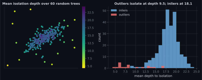
• measured separation: outliers isolate at depth 9.46, inliers at 18.09
• why max_samples=256max_samples=256 is the default and why subsampling improves accuracy here
• contaminationcontamination as a threshold, not a model — the precision/recall curve it traces
• four detectors on identical data: 16, 17, 13 and 18 correct out of 20
• when to use Isolation Forest, and the three situations where it is the wrong tool

Intuition

Most anomaly detection tries to build a model of “normal” and then flags whatever the model fits badly. That is expensive: you have to characterise the bulk of the data precisely, and the bulk is where nearly all the data is.

Isolation Forest inverts the problem. It observes that anomalies are few and different, and that those two properties make them easy to separate from everything else. So instead of describing normality, it repeatedly cuts the feature space at random and asks a much cheaper question: how many cuts did it take before this point ended up alone?

A point in the middle of a dense cloud is surrounded, so a random cut is unlikely to separate it from its neighbours — it takes many cuts. A point sitting far out on its own gets sliced off almost immediately. Short path to isolation means anomalous.

The consequence is unusual and worth appreciating: this algorithm never computes a distance, never estimates a density, and never looks at the whole dataset. It is the rare case where the anomaly detector is cheaper than the thing it is detecting anomalies in.

  flowchart TD
  A["Subsample 256 rows"] --> B["Pick a random feature"]
  B --> C["Pick a random split value
between that feature's min and max"]
  C --> D{"Is the target point alone
in its region?"}
  D -->|"no"| B
  D -->|"yes"| E["Record the depth"]
  E --> F["Average over 100 trees"]
  F --> G["Short average depth -> anomaly
Long average depth -> normal"]

The math

An isolation tree is built by recursively choosing a random feature $q$ and a random split value $p$ uniformly between the current node’s minimum and maximum of $q$, until every point is alone or a height limit is hit.

Write $h(x)$ for the path length of point $x$ — the number of edges from the root to its terminating node.

Path length alone is not comparable across dataset sizes: a tree over 10,000 points is deeper than one over 100 points, for everyone. The normalisation comes from the fact that an isolation tree is structurally a binary search tree, and the average unsuccessful-search path length in a BST over $n$ nodes is known:

where $\gamma$ is the Euler-Mascheroni constant. Dividing by $c(n)$ makes depths comparable. The anomaly score is then

where $E[h(x)]$ is the average path length over all the trees. Read the three regimes off the exponent:

With $n = 256$:

So a point isolated at average depth 4 scores $2^{-4/10.2448} = 0.7629$, at depth 10.2448 scores exactly $0.5$, and at depth 14 scores $0.3878$.

scikit-learn flips the sign. Its score_samplesscore_samples returns the negative of the above, so lower is more anomalous and the values are negative. decision_functiondecision_function is score_samples - offset_score_samples - offset_, which puts the decision boundary at zero. Getting this backwards is the single most common bug with this estimator.

Why subsample?

The default max_samples=256max_samples=256 is not a speed compromise — it makes the detector more accurate. Two effects work against large samples:

• Swamping: with many points, normal points near a cluster of anomalies get dragged into looking anomalous.
• Masking: a dense clump of anomalies looks like a legitimate small cluster and stops being isolated quickly.

Subsampling breaks up both. Each tree sees a different 256 rows, so an anomaly clump rarely survives intact in any one of them. The original paper found accuracy plateaus around 256 and adding more rows does not help — which is why the parameter is a fixed count, not a fraction.

Worked example by hand

Six points on a line: $1, 2, 3, 4, 5, 20$. The value 20 is the obvious anomaly.

Build one isolation tree. The root spans $[1, 20]$. Draw a random split $p \sim U(1, 20)$.

The point 20 is isolated at depth 1 whenever $p > 5$ — probability $(20 - 5)/(20 - 1) = 15/19 = 0.789$. Four times out of five, one cut is enough.

The point 3 can never be isolated at depth 1. It has neighbours on both sides, so any single split leaves it with company: $p \in (2, 3)$ gives $\{3, 4, 5, 20\}$ on the right, and $p \in (3, 4)$ gives $\{1, 2, 3\}$ on the left. Its shortest possible path is 2, and typically it is much longer.

Averaging over 4,000 random trees:

With $n = 6$:

So 20 scores $2^{-1.222/2.7066} = 0.7314$ while 3 scores $2^{-5.952/2.7066} = 0.2178$. Comfortably above and comfortably below 0.5 — exactly the split the score is designed to produce.

Note that the two edge points, 1 and 5, score higher than the interior ones. That is correct behaviour, not an artefact: being at the edge of the range genuinely does make you easier to isolate, and every isolation-based method inherits this mild edge bias.

Scaled up to 300 points in two dimensions — 280 from a correlated Gaussian and 20 uniform outliers — the separation is unambiguous:

figureIsolation depth separates the two populationsmatplotlib

See it move

The next sketch shows the scoring formula directly: drag through the depth axis and watch $s$ cross 0.5 exactly where $E[h] = c(n)$.

Notice how little $c(n)$ moves: 64 rows give 7.72, 4096 give 15.79. Path length grows roughly logarithmically in $n$, which is exactly why the normalisation is a logarithm.

contamination is a threshold, not a model

contaminationcontamination does not change a single tree. It only decides where to cut the score distribution — it sets offset_offset_ to the corresponding quantile. Getting it wrong therefore costs you nothing in model quality and everything in what comes out.

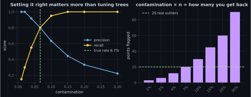
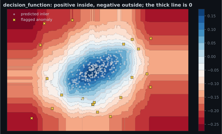
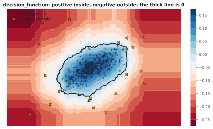
On 300 points containing 20 genuine outliers (a true rate of 6.67%):

The number flagged is exactly round(contamination × n)round(contamination × n) in every row — the parameter is a quota, not a discovery. Setting it to the true rate balances precision and recall at 0.80 each.

figureOne parameter, one trade-offmatplotlib

The underlying ranking is excellent regardless: the ROC AUC of the raw scores is 0.9902. The model knows which points are odd. contaminationcontamination only decides how many of them you are told about.

figureThe decision function across the whole planematplotlib

Four detectors, one dataset

Same 300 points, same 20 planted outliers, same 7% budget:

figureFour detectors on identical datamatplotlib

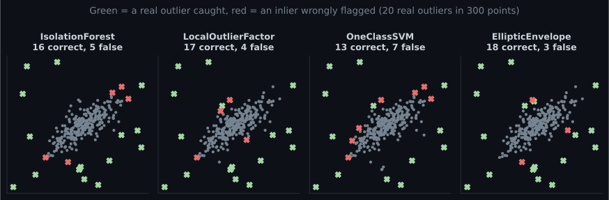
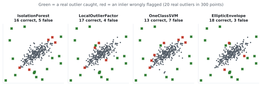
That result is worth stating plainly: the best detector on this page is not Isolation Forest. EllipticEnvelope wins because the data was generated from a bivariate Gaussian and it fits a bivariate Gaussian. That is a property of the benchmark, not evidence of general superiority — and it is the reason to be suspicious of any anomaly-detection comparison, including this one.

Isolation Forest’s case is different: it makes no distributional assumption, scales to millions of rows, handles dozens of features, and has essentially nothing to tune. On real data where you do not know the shape of “normal”, those properties matter more than two extra hits on a synthetic benchmark.

In code

import numpy as np
from sklearn.ensemble import IsolationForest
 
rng = np.random.default_rng(3)
cov = np.array([[1.0, 0.75], [0.75, 1.0]])
inliers = rng.multivariate_normal([0, 0], cov, size=280)
outliers = rng.uniform(-5, 5, size=(20, 2))
X = np.vstack([inliers, outliers])
 
clf = IsolationForest(
    n_estimators=100,      # more trees = more stable scores, no overfitting risk
    max_samples=256,       # the paper's default; subsampling improves accuracy
    contamination=0.07,    # a THRESHOLD, not a model parameter
    random_state=0,
).fit(X)
 
pred = clf.predict(X)              # +1 inlier, -1 outlier
scores = clf.score_samples(X)      # LOWER is more anomalous (sklearn flips the sign)
margin = clf.decision_function(X)  # score_samples - offset_; negative means flagged
 
print("flagged        ", int((pred == -1).sum()))         # 21
print("offset_        ", round(clf.offset_, 4))           # -0.5382
print("inlier  mean s ", round(scores[:280].mean(), 4))   # -0.4212
print("outlier mean s ", round(scores[280:].mean(), 4))   # -0.6387

import numpy as np
from sklearn.ensemble import IsolationForest
 
rng = np.random.default_rng(3)
cov = np.array([[1.0, 0.75], [0.75, 1.0]])
inliers = rng.multivariate_normal([0, 0], cov, size=280)
outliers = rng.uniform(-5, 5, size=(20, 2))
X = np.vstack([inliers, outliers])
 
clf = IsolationForest(
    n_estimators=100,      # more trees = more stable scores, no overfitting risk
    max_samples=256,       # the paper's default; subsampling improves accuracy
    contamination=0.07,    # a THRESHOLD, not a model parameter
    random_state=0,
).fit(X)
 
pred = clf.predict(X)              # +1 inlier, -1 outlier
scores = clf.score_samples(X)      # LOWER is more anomalous (sklearn flips the sign)
margin = clf.decision_function(X)  # score_samples - offset_; negative means flagged
 
print("flagged        ", int((pred == -1).sum()))         # 21
print("offset_        ", round(clf.offset_, 4))           # -0.5382
print("inlier  mean s ", round(scores[:280].mean(), 4))   # -0.4212
print("outlier mean s ", round(scores[280:].mean(), 4))   # -0.6387

Ranking beats thresholding whenever a human is going to look at the results anyway:

import numpy as np
 
# Forget contamination — hand the analyst the 20 oddest rows.
order = np.argsort(clf.score_samples(X))     # most anomalous first
top20 = order[:20]
print("indices of the 20 most anomalous rows:", top20)
 
# How many were real? (Only knowable here because we planted them.)
print("hits in the top 20:", int((top20 >= 280).sum()))

import numpy as np
 
# Forget contamination — hand the analyst the 20 oddest rows.
order = np.argsort(clf.score_samples(X))     # most anomalous first
top20 = order[:20]
print("indices of the 20 most anomalous rows:", top20)
 
# How many were real? (Only knowable here because we planted them.)
print("hits in the top 20:", int((top20 >= 280).sum()))

And when you genuinely have labels, measure the ranking rather than the threshold:

from sklearn.metrics import average_precision_score, roc_auc_score
 
y_true = np.concatenate([np.zeros(280), np.ones(20)])    # 1 = outlier
y_score = -clf.score_samples(X)                          # flip so higher = more anomalous
 
print("ROC AUC", round(roc_auc_score(y_true, y_score), 4))            # 0.9902
print("PR AUC ", round(average_precision_score(y_true, y_score), 4))

from sklearn.metrics import average_precision_score, roc_auc_score
 
y_true = np.concatenate([np.zeros(280), np.ones(20)])    # 1 = outlier
y_score = -clf.score_samples(X)                          # flip so higher = more anomalous
 
print("ROC AUC", round(roc_auc_score(y_true, y_score), 4))            # 0.9902
print("PR AUC ", round(average_precision_score(y_true, y_score), 4))

With 6.7% positives, average precision is the more honest number — ROC AUC flatters imbalanced problems, exactly as it does in supervised classification.

Novelty detection versus outlier detection

Two different jobs that use the same estimators:

Outlier detection — the training set is already contaminated, and you want to know which of these rows are odd. fit_predict(X)fit_predict(X).

Novelty detection — the training set is clean, and you want to flag odd rows in future data. fit(X_clean)fit(X_clean) then predict(X_new)predict(X_new).

Isolation Forest supports both directly. LocalOutlierFactorLocalOutlierFactor requires novelty=Truenovelty=True at construction time and then forbids fit_predictfit_predict — a common source of confusion.

Pitfalls

Getting the sign backwards. In the paper, higher $s$ means more anomalous. In scikit-learn, score_samplesscore_samples is negated, so lower means more anomalous. Flip it before feeding roc_auc_scoreroc_auc_score, or your AUC will come out near 0.01 instead of 0.99.

Treating contaminationcontamination as tuning. It changes nothing about the trees. The sweep above shows it moving precision from 1.00 to 0.22 while the underlying ranking (AUC 0.9902) is unchanged throughout.

Raising max_samplesmax_samples to “use all the data”. Subsampling is a feature. Large samples reintroduce swamping and masking, which is what the 256 default exists to prevent.

Expecting it to find contextual anomalies. A temperature of 30°C is normal in July and bizarre in January. Isolation Forest sees only the marginal distribution unless you engineer the context into a feature (temp_minus_monthly_meantemp_minus_monthly_mean).

Using it on categorical data. Random splits on a one-hot column are almost meaningless — the “range” of a binary column is $[0, 1]$ and any cut is the same cut. Encode ordinally with a meaningful order, or use a method built for mixed types.

Ignoring that some anomalies are unfindable. In the measured data, several uniform outliers landed inside the Gaussian cloud. No unsupervised detector can flag those, and chasing them by raising contamination only buys false alarms — precision fell from 1.00 to 0.44 to recover the last few.

Assuming it beats the alternatives. It lost to EllipticEnvelope 18–16 on this page’s Gaussian data. Benchmark on your data.

Compare

Isolation Forest not needing scaling is genuinely unusual and follows from the splits being per-feature: a cut is drawn uniformly within each feature’s own range, so the units cancel.

🧪 Try It Yourself

Exercise 1 – The normalisation constant

Exercise 2 – Fit one and read the scores

Exercise 3 – contamination is a quota

Exercise 4 – Rank instead of threshold

Exercise 5 – Four detectors, one dataset

Recap

• Isolation Forest finds anomalies by how easily they are separated, not by modelling normality.
• The score $s = 2^{-E[h]/c(n)}$ uses the average BST path length $c(n)$ so depths are comparable across dataset sizes. $c(256) = 10.2448$, and $E[h] = c(n)$ gives exactly $s = 0.5$.
• Measured separation: outliers isolate at mean depth 9.46, inliers at 18.09.
• Subsampling to 256 rows per tree is an accuracy improvement, not a compromise — it defeats swamping and masking.
• contaminationcontamination is a quantile threshold. It flagged exactly $\text{round}(c \times n)$ points at every setting while the ranking’s ROC AUC stayed at 0.9902.
• scikit-learn negates the score: lower score_samplesscore_samples means more anomalous.
• On this page’s Gaussian benchmark, EllipticEnvelope won 18–16. That reflects the benchmark, and it is the reason to test on your own data.

Exercise 6 – contaminationcontamination is a review budget

Next

Association Rule Learning (Apriori Algorithm) — a different kind of unsupervised structure entirely: not “which rows are alike?” but “which items show up together, and is that more often than chance?”