
Gradient Descent Explained
What you’ll learn
Section titled “What you’ll learn”- the update rule , derived rather than asserted
- two full iterations computed by hand, matching NumPy to four decimals
- the exact threshold at which a learning rate stops converging and starts exploding
- batch, stochastic and mini-batch descent — the real trade-off between them
- why feature scaling turns a slow ravine into a fast bowl
- learning schedules, and when to stop
Intuition
Section titled “Intuition”You are standing on a hillside in fog. You cannot see the valley floor, but you can feel which way the ground slopes under your feet. Take a step downhill. Feel again. Step again.
That is the entire algorithm. The gradient is the direction of steepest ascent, so you move against it. The learning rate is how long a stride you take. Everything else — momentum, Adam, schedules — is refinement of those two sentences.
  flowchart TD
  A["Start from random parameters"] --> B["Compute predictions"]
  B --> C["Compute cost J"]
  C --> D["Compute gradient of J"]
  D --> E["Step against the gradient"]
  E --> F{"Converged?"}
  F -->|no| B
  F -->|yes| G["Return theta"]
The Normal Equation from Multiple Linear Regression already solves linear regression exactly, so why iterate at all? Because inverting an matrix costs roughly . At 100,000 features that is hopeless, and for models with no closed form at all — logistic regression, neural networks, gradient boosting — iteration is the only option. Gradient descent is the workhorse of the entire field; linear regression is just the clearest place to learn it.
The math
Section titled “The math”The update rule
Section titled “The update rule”For a cost , the gradient collects the partial derivatives:
and each iteration steps against it:
is the learning rate. It is the only hyperparameter, and it decides everything.
The gradient of MSE
Section titled “The gradient of MSE”With , differentiating gives a strikingly simple result:
Read it as English: the residual vector, projected back onto the features, scaled by two over the sample count. Every feature gets pushed in proportion to how much it contributed to the current error.
When does it actually converge?
Section titled “When does it actually converge?”This is the part most tutorials skip. For a quadratic cost with Hessian , gradient descent converges if and only if
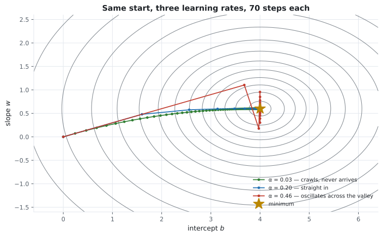
where is the largest eigenvalue. Above that threshold each step overshoots by more than it corrects and the parameters diverge geometrically. The condition number then decides how fast convergence happens: a of 1 is a round bowl and descent goes straight in, while a of 1,000 is a narrow ravine that forces a zig-zag.
Both facts have the same practical consequence, and it is the reason for the whole preprocessing phase: scale your features.
Worked example by hand
Section titled “Worked example by hand”The five-point dataset with the feature centred (), so the Hessian is diagonal and the arithmetic stays exact. Parameters are , starting from , with .
| 1 | −2 | 2 |
| 2 | −1 | 4 |
| 3 | 0 | 5 |
| 4 | 1 | 4 |
| 5 | 2 | 5 |
The Hessian, and the stability limit.
Eigenvalues 2 and 4, so descent diverges for any . Our 0.2 is comfortably inside. The optimum is .
Iteration 0. With every prediction is 0, so the residual is :
Iteration 1. Predictions are now , giving residuals :
The cost falling.
| step | MSE | ||
|---|---|---|---|
| 0 | 0.000 | 0.0000 | 17.2000 |
| 1 | 1.600 | 0.4800 | 6.2688 |
| 2 | 2.560 | 0.5760 | 2.5548 |
| 3 | 3.136 | 0.5952 | 1.2265 |
| ⋮ | ⋮ | ⋮ | ⋮ |
| ∞ | 4.000 | 0.6000 | 0.4800 |
The slope reaches its final value almost immediately while the intercept takes far longer. That is the condition number in action: the eigenvalue along is twice the eigenvalue along , so the same makes twice the progress in that direction.
The learning rate
Section titled “The learning rate”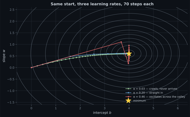
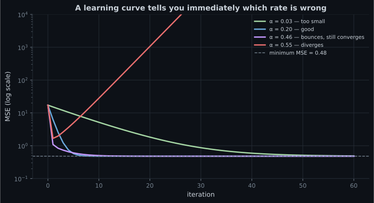
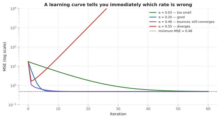
Reading the plots
Section titled “Reading the plots”| What you see | What it means | What to do |
|---|---|---|
| Cost falls smoothly to a plateau | Healthy | Nothing |
| Cost falls, very slowly | too small | Multiply by 3 |
| Cost oscillates but trends down | just under the limit | Halve it |
Cost rises or hits nan | above | Divide by 10 |
| Cost falls then flattens high | Underfitting, not an problem | More features or capacity |
A practical recipe: try , plot all four cost curves on one log axis, and take the largest rate that still descends smoothly.
Notice the steps shrinking on their own as the curve flattens. The learning rate never changes — the gradient shrinks near the minimum, so descent automatically slows down as it arrives.
Why scaling matters
Section titled “Why scaling matters”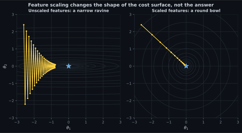
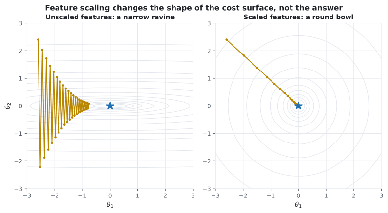
Unscaled features produce an elongated cost surface, and the negative gradient points across the valley rather than down it. Standardising makes the contours near-circular and lets descent walk straight in — often an order of magnitude fewer iterations, from the same code.
from sklearn.datasets import load_diabetes
from sklearn.linear_model import SGDRegressor
from sklearn.model_selection import train_test_split
from sklearn.pipeline import make_pipeline
from sklearn.preprocessing import StandardScaler

X, y = load_diabetes(return_X_y=True)
X_train, X_test, y_train, y_test = train_test_split(
    X, y, test_size=0.3, random_state=42
)

scaled = make_pipeline(
    StandardScaler(),
    SGDRegressor(max_iter=2000, tol=1e-4, eta0=0.01, random_state=0),
).fit(X_train, y_train)

raw = SGDRegressor(
    max_iter=2000, tol=1e-4, eta0=0.01, random_state=0
).fit(X_train, y_train)

print(f"scaled   R^2 = {scaled.score(X_test, y_test):.4f}")  # 0.4767
print(f"unscaled R^2 = {raw.score(X_test, y_test):.4f}")     # 0.4554
print(f"epochs used  = {scaled[-1].n_iter_}")                # 27
The scaled pipeline converges in 27 epochs and lands on 0.4767 — indistinguishable from the exact Normal Equation answer of 0.4773. The unscaled version burns all 2,000 epochs, emits a convergence warning, and still ends up worse.
The three variants
Section titled “The three variants”How much data does one gradient use?
  flowchart TD
  A["Batch GD
all m rows per step"] --> A2["Smooth, expensive steps
settles exactly on the minimum"]
  B["Stochastic GD
1 random row per step"] --> B2["Cheap, noisy steps
bounces around the minimum forever"]
  C["Mini-batch GD
32 to 256 rows per step"] --> C2["Balanced; vectorises well on GPUs
the default everywhere"]
The stochastic gradient is an unbiased estimate of the batch gradient — right on average, wrong on any individual step. That noise is not purely a cost: it lets SGD escape shallow local minima that would trap batch descent on non-convex problems, which is exactly why deep learning uses it.
| Batch | Stochastic | Mini-batch | |
|---|---|---|---|
| Rows per step | 1 | 32–256 | |
| Cost per step | High | Very low | Low |
| Path | Smooth | Very noisy | Slightly noisy |
| Settles exactly? | Yes | No, needs a schedule | Nearly |
| Out-of-core | No | Yes | Yes |
| Hardware fit | Poor | Poor | Excellent |
| scikit-learn | LinearRegression | SGDRegressor | SGDRegressor.partial_fit |
Learning schedules
Section titled “Learning schedules”Because SGD never settles, the standard fix is to shrink the learning rate over time:
Early on the steps are long enough to cover ground; later they are short enough to sit still. Decay
too fast and it freezes before arriving; too slowly and it keeps bouncing. SGDRegressor exposes
this as learning_rate="invscaling" with eta0 and power_t.
From scratch
Section titled “From scratch”import numpy as np
def batch_gradient_descent(X, y, lr=0.2, n_iter=50):
"""Plain batch gradient descent. X must already include the bias column."""
m = len(y)
theta = np.zeros(X.shape[1])
history = []
for _ in range(n_iter):
residual = X @ theta - y
history.append(float((residual**2).mean()))
gradient = (2 / m) * X.T @ residual
theta = theta - lr * gradient
return theta, history
x_centred = np.array([1.0, 2.0, 3.0, 4.0, 5.0]) - 3.0
X = np.c_[np.ones(5), x_centred]
y = np.array([2.0, 4.0, 5.0, 4.0, 5.0])
theta, history = batch_gradient_descent(X, y, lr=0.2, n_iter=50)
print(theta.round(4)) # [4. 0.6]
print([round(h, 4) for h in history[:4]])
# [17.2, 6.2688, 2.5548, 1.2265]
# The stability limit, computed rather than guessed
hessian = (2 / len(y)) * X.T @ X
print(f"max stable lr = {2 / np.linalg.eigvalsh(hessian).max():.3f}") # 0.500The first four cost values reproduce the hand-computed table exactly, and after 50 iterations the parameters have reached the Normal Equation’s answer of .
pch.algoApi sklearn.linear_model.SGDRegressor (stochastic and mini-batch variants)
pch.algoAssumes
- The cost is differentiable with respect to the parameters
- The learning rate is below 2 over the largest Hessian eigenvalue
- Features are on comparable scales, or convergence will be slow
pch.algoCost
- pch.algoTrain
O(m·n) per iteration- pch.algoPredict
O(n)- pch.algoMemory
O(n)
m = samples, n = features; total cost is per-iteration cost times the iteration count
pch.algoHyperparams
-
learning_rate (alpha, eta0)default 0.01 The one that matters. Too small crawls, too large diverges. Tune on a log grid. -
max_iterdefault 1000 Iteration budget. Pair it with tol so training stops when progress stalls. -
toldefault 1e-3 Stop when the loss improves by less than this for n_iter_no_change epochs. -
batch sizedefault 1 for SGDRegressor Larger batches mean smoother gradients and better hardware use; 32 to 256 is the usual range.
pch.algoReachFor
- You have too many features for a closed-form solution
- The data does not fit in memory and must stream
- The model has no closed form at all — logistic regression, neural networks
- You want to warm-start or update a model online
pch.algoLookElsewhere
- The problem is small and a closed form exists — just use LinearRegression
- You cannot scale the features
- You need bit-for-bit reproducibility without pinning every random seed
Pitfalls
Section titled “Pitfalls”-
Why does the update rule subtract the gradient instead of adding it?
The gradient is the direction of steepest ascent. Minimising means walking the other way.
pch.quizShowAnswer
B — Because the gradient points in the direction of steepest increase, and we want to decrease the cost — The gradient is the direction of steepest ascent. Minimising means walking the other way.
-
Your cost becomes nan after four iterations. What is the most likely cause?
Above 2 divided by the largest Hessian eigenvalue, the iteration diverges geometrically and overflows within a few steps. Reduce the learning rate by a factor of ten.
pch.quizShowAnswer
B — The learning rate exceeds the stability threshold, so each step overshoots more than the last — Above 2 divided by the largest Hessian eigenvalue, the iteration diverges geometrically and overflows within a few steps. Reduce the learning rate by a factor of ten.
-
What is the practical effect of feature scaling on gradient descent?
Scaling does not change where the minimum is in terms of predictions — it changes the shape of the path to it. Rounder contours mean the negative gradient points at the minimum instead of across the valley.
pch.quizShowAnswer
B — It makes the cost contours rounder, so descent needs far fewer iterations to reach the same minimum — Scaling does not change where the minimum is in terms of predictions — it changes the shape of the path to it. Rounder contours mean the negative gradient points at the minimum instead of across the valley.
-
Why does stochastic gradient descent still work despite using one row per step?
Each step is wrong individually but right on average. Over many cheap steps the errors cancel, and the noise even helps escape shallow minima on non-convex problems.
pch.quizShowAnswer
B — Because the single-row gradient is an unbiased estimate of the full gradient, so the noise averages out over many steps — Each step is wrong individually but right on average. Over many cheap steps the errors cancel, and the noise even helps escape shallow minima on non-convex problems.
🧪 Try It Yourself
Section titled “🧪 Try It Yourself”Exercise 1 – One batch gradient step
Section titled “Exercise 1 – One batch gradient step”Exercise 2 – Watch the cost fall
Section titled “Exercise 2 – Watch the cost fall”Exercise 3 – Compute the stability limit
Section titled “Exercise 3 – Compute the stability limit”Exercise 4 – Push it past the limit
Section titled “Exercise 4 – Push it past the limit”Exercise 5 – Scaling changes everything for SGD
Section titled “Exercise 5 – Scaling changes everything for SGD”- The update rule is , and for MSE the gradient is .
- Convergence requires — on the worked example, 0.5.
- Two hand iterations at take the cost from 17.20 to 6.27 to 2.55, matching NumPy exactly.
- Scaling controls the condition number, which controls how many iterations you pay for.
- Batch is smooth and expensive, stochastic is noisy and cheap, mini-batch is the default.
- Plot cost against iteration on every run; the shape of that curve diagnoses the learning rate immediately.
Exercise 6 – Find the learning rate that breaks it
Section titled “Exercise 6 – Find the learning rate that breaks it”Continue to Regularization - Ridge and Lasso Regression — add a penalty term to the same cost and watch overfitting recede.
pch.coffeeTagline
pch.coffeeCtapch.feedbackHeading
pch.feedbackSubheading