Angles and Orthogonality

Cauchy-Schwarz guaranteed that

$$\frac{\langle\mathbf{x},\mathbf{y}\rangle}{\lVert\mathbf{x}\rVert\,\lVert\mathbf{y}\rVert} \in [-1,\ 1] .$$

A number in that range can be called a cosine, and that single move gives the inner product a geometric meaning: it measures angle. From there come cosine similarity — the standard way to compare embeddings — and orthogonality, which every remaining page of this chapter is built on.

The page also carries the chapter’s most important caveat, and it is worth stating up front: orthogonality is a statement about a pair of vectors and an inner product, not about the pair alone.

What you’ll learn

• The definition of the angle $\omega$ between two vectors, and why the normalisation matters more than the numerator.
• Cosine similarity, and a measured demonstration of what goes wrong if you use the raw dot product instead.
• Orthogonality (Definition 3.7), including the fact that $\mathbf{0}$ is orthogonal to everything.
• The book’s Example 3.7: a pair at $90°$ under the dot product and at $109.47°$ under a different inner product — same two arrows.
• Orthogonal matrices (Definition 3.8), the two properties that make them the transformations of choice, and why the book says “orthonormal” would be the better word.
• Why two random high-dimensional vectors are almost always nearly perpendicular, measured across four orders of magnitude of dimension.

Intuition: the numerator says how much, the denominator says compared to what

The dot product $\mathbf{x}^\top\mathbf{y}$ conflates two different questions: do these point the same way? and how big are they? Two long documents about unrelated topics can share a large dot product purely by being long.

Dividing by both lengths removes the second question entirely. What is left is scale-free — multiply either vector by any positive number and the cosine does not move — and so it answers only the first question. That is why every retrieval system compares embeddings by cosine and not by dot product, unless the embeddings have already been normalised, in which case the two coincide.

diagram Diagram mermaid

  flowchart TD
  IP["⟨x, y⟩
large when aligned AND when long"]
  IP --> DIV["divide by ‖x‖ ‖y‖"]
  DIV --> COS["cos ω ∈ [−1, 1]
scale-free: only direction is left"]
  COS --> POS["cos ω > 0
acute: pointing broadly together"]
  COS --> ZERO["cos ω = 0
ORTHOGONAL, Def 3.7"]
  COS --> NEG["cos ω < 0
obtuse: pointing broadly apart"]
  ZERO --> ONB["an orthonormal basis
§3.5"]
  ZERO --> PROJ["projections
§3.8"]
  COS --> REL["but which inner product?
Example 3.7: the SAME pair is
90° under one and 109.47° under another"]

The math

The angle

Equations 3.24 and 3.25 — the angle between two vectors

For $\mathbf{x}, \mathbf{y} \neq \mathbf{0}$, the angle $\omega \in [0, \pi]$ between them is defined by

$$\cos\omega = \frac{\langle \mathbf{x}, \mathbf{y}\rangle}{\lVert\mathbf{x}\rVert\,\lVert\mathbf{y}\rVert}, \qquad \omega = \arccos\!\left(\frac{\langle \mathbf{x}, \mathbf{y}\rangle}{\lVert\mathbf{x}\rVert\,\lVert\mathbf{y}\rVert}\right)$$

This is well defined because Cauchy-Schwarz confines the argument to $[-1,1]$, and unique because $\arccos$ is a bijection from $[-1,1]$ to $[0,\pi]$.

The restriction $\omega \in [0,\pi]$ is worth noticing: this is an unsigned angle. There is no orientation and no “clockwise” — the angle from $\mathbf{x}$ to $\mathbf{y}$ equals the angle from $\mathbf{y}$ to $\mathbf{x}$, because the inner product is symmetric.

Orthogonality

Definition 3.7 — Orthogonality

Two vectors $\mathbf{x}$ and $\mathbf{y}$ are orthogonal if and only if $\langle \mathbf{x}, \mathbf{y}\rangle = 0$, written $\mathbf{x} \perp \mathbf{y}$. If additionally $\lVert\mathbf{x}\rVert = \lVert\mathbf{y}\rVert = 1$ — both are unit vectors — then $\mathbf{x}$ and $\mathbf{y}$ are orthonormal.

The zero vector is orthogonal to everything in the space.

Three things about that definition.

It is defined by the inner product being zero, not by the angle being $90°$. The two agree for nonzero vectors, but the inner-product form also covers $\mathbf{0}$, whose angle with anything is undefined (you would be dividing by zero) while its inner product with everything is $0$.

It is relative. The definition names an inner product, and different inner products give different answers on the same pair. The next section is the book’s own demonstration.

Orthonormal is orthogonal plus unit length. The distinction matters from §3.5 onwards, where the unit-length half is what makes coordinates cheap.

Orthogonal matrices

Definition 3.8 — Orthogonal matrix

A square matrix $\mathbf{A}$ is orthogonal if and only if its columns are orthonormal, so that

$$\mathbf{A}\mathbf{A}^\top = \mathbf{I} = \mathbf{A}^\top\mathbf{A}, \qquad\text{which implies}\qquad \mathbf{A}^{-1} = \mathbf{A}^\top .$$

The inverse being the transpose is worth its own line, because it is the reason orthogonal matrices are everywhere in numerical code: inverting one is free, and free inversion means no conditioning problem.

Two consequences, both of which the book states:

Lengths are preserved (Equation 3.31):

$$\lVert\mathbf{A}\mathbf{x}\rVert^2 = (\mathbf{A}\mathbf{x})^\top(\mathbf{A}\mathbf{x}) = \mathbf{x}^\top\mathbf{A}^\top\mathbf{A}\mathbf{x} = \mathbf{x}^\top\mathbf{I}\mathbf{x} = \mathbf{x}^\top\mathbf{x} = \lVert\mathbf{x}\rVert^2$$

Angles are preserved (Equation 3.32):

$$\cos\omega = \frac{(\mathbf{A}\mathbf{x})^\top(\mathbf{A}\mathbf{y})}{\lVert\mathbf{A}\mathbf{x}\rVert\lVert\mathbf{A}\mathbf{y}\rVert} = \frac{\mathbf{x}^\top\mathbf{A}^\top\mathbf{A}\mathbf{y}}{\lVert\mathbf{x}\rVert\lVert\mathbf{y}\rVert} = \frac{\mathbf{x}^\top\mathbf{y}}{\lVert\mathbf{x}\rVert\lVert\mathbf{y}\rVert}$$

Every step in both derivations is the substitution $\mathbf{A}^\top\mathbf{A} = \mathbf{I}$. So an orthogonal matrix is exactly a map that leaves all of Euclidean geometry alone — the transformations that “do not change anything” in the sense that matters here. §3.9 will name the determinant-$+1$ half of them rotations; the other half are reflections.

The book’s own terminology complaint

The book notes in a margin that these matrices should really be called orthonormal, since the definition requires the columns to be orthogonal and of unit length. “Orthogonal matrix” is the universal name anyway, so both the book and this page use it — but if you ever wonder why $\mathbf{A}^\top\mathbf{A} = \mathbf{I}$ rather than merely a diagonal matrix, this is why.

From the book

Section 3.4. The angle is Equations 3.24 and 3.25, illustrated by Figure 3.4. Example 3.6 (Equation 3.26) computes the angle between $(1,1)^\top$ and $(1,2)^\top$; Figure 3.5 draws it. Definition 3.7 gives orthogonality and orthonormality, Example 3.7 (Equations 3.27 and 3.28) the inner-product dependence with Figure 3.6, and Definition 3.8 the orthogonal matrix (Equations 3.29 and 3.30) with Equations 3.31 and 3.32 for the two preservation properties.

Worked example by hand

Example 3.6 from the book

$\mathbf{x} = (1,1)^\top$, $\mathbf{y} = (1,2)^\top$, dot product.

quantity	working	value
$\langle\mathbf{x},\mathbf{y}\rangle$	$1\cdot1 + 1\cdot2$	$3$
$\lVert\mathbf{x}\rVert$	$\sqrt{1+1}$	$\sqrt{2} \approx 1.414214$
$\lVert\mathbf{y}\rVert$	$\sqrt{1+4}$	$\sqrt{5} \approx 2.236068$
$\cos\omega$	$\dfrac{3}{\sqrt{2}\sqrt{5}} = \dfrac{3}{\sqrt{10}}$	$0.948683$
$\omega$	$\arccos(0.948683)$	$0.321751$ rad $= 18.434949°$

The book quotes $\cos\omega = 3/\sqrt{10}$ and $\omega \approx 0.32$ rad $\approx 18°$, which the exact values confirm.

Example 3.7 — the one to remember

$\mathbf{x} = (1,1)^\top$, $\mathbf{y} = (-1,1)^\top$.

Under the dot product: $\langle\mathbf{x},\mathbf{y}\rangle = -1 + 1 = 0$, so $\cos\omega = 0$ and $\omega = 90°$ exactly. Orthogonal.

Under $\langle\mathbf{x},\mathbf{y}\rangle = \mathbf{x}^\top\begin{bmatrix}2&0\\0&1\end{bmatrix}\mathbf{y}$:

$$\langle\mathbf{x},\mathbf{y}\rangle = 2(1)(-1) + 1(1)(1) = -2 + 1 = -1$$ $$\lVert\mathbf{x}\rVert = \sqrt{2(1) + 1(1)} = \sqrt{3}, \qquad \lVert\mathbf{y}\rVert = \sqrt{2(1) + 1(1)} = \sqrt{3}$$ $$\cos\omega = \frac{-1}{\sqrt{3}\cdot\sqrt{3}} = -\frac{1}{3} \approx -0.333333, \qquad \omega = 1.910633\ \text{rad} = 109.4712°$$

The book quotes $\omega \approx 1.91$ rad $\approx 109.5°$. Same two arrows on the same piece of paper; one geometry says they meet at a right angle and the other says they meet at $109.47°$ — which happens to be the tetrahedral angle, though that is a coincidence here.

The mechanism is visible in the numbers: the matrix $\mathrm{diag}(2,1)$ makes the $x_1$ direction count double, and $\mathbf{x}$ and $\mathbf{y}$ have $x_1$ components of opposite sign. Weighting that disagreement more heavily tips the total negative.

examples_36_37.py

import numpy as np
 
x = np.array([1.0, 1.0])
y = np.array([1.0, 2.0])
c = float(x @ y) / (np.linalg.norm(x) * np.linalg.norm(y))
print("Example 3.6: cos =", c, " = 3/sqrt(10) ?", np.isclose(c, 3 / np.sqrt(10)))
print("             omega =", np.arccos(c), "rad =", np.degrees(np.arccos(c)), "deg")
 
y2 = np.array([-1.0, 1.0])
for name, A in (("dot product", np.eye(2)), ("diag(2, 1)", np.diag([2.0, 1.0]))):
    ip = float(x @ A @ y2)
    cc = ip / np.sqrt(float(x @ A @ x) * float(y2 @ A @ y2))
    print(f"Example 3.7 under {name:12}: <x,y> = {ip:+.4f}  cos = {cc:+.6f}  "
          f"omega = {np.degrees(np.arccos(cc)):.4f} deg")

output

Example 3.6: cos = 0.9486832980505138  = 3/sqrt(10) ? True
             omega = 0.3217505543966423 rad = 18.434948822922017 deg
Example 3.7 under dot product : <x,y> = +0.0000  cos = +0.000000  omega = 90.0000 deg
Example 3.7 under diag(2, 1)  : <x,y> = -1.0000  cos = -0.333333  omega = 109.4712 deg

See it move

The first sketch separates the two questions the dot product conflates. Drag $\mathbf{y}$‘s direction and the cosine changes; drag its length and the cosine does not move at all while the raw inner product does.

sketch Length changes the dot product and not the cosine p5.js Pause Restart

Drag the blue arrow to change direction, and drag the length knob to change its magnitude. The arc and the cosine readout depend only on direction; the raw inner product depends on both. That difference is the entire reason cosine similarity exists.

The second sketch is Example 3.7 on a knob. Both arrows stay exactly where they are while the geometry moves out from under them.

sketch Example 3.7: the same pair, 90 degrees or 109.47 p5.js Pause Restart

The two arrows are fixed at (1,1) and (-1,1). The knob is the top-left entry of diag(a, 1) — the weight given to the first coordinate. At a = 1 the inner product is the dot product and the vectors are orthogonal. At a = 2 the book's second inner product gives cos = -1/3 and 109.4712 degrees. The dashed ellipse is the unit set, and it is what is actually changing.

The third checks Definition 3.8’s two claims by applying a transformation and remeasuring.

sketch Orthogonal matrices leave lengths and angles alone p5.js Pause Restart

Drag theta to rotate, and drag the reflect knob to flip the sign of the second column. Both give an orthogonal matrix — determinant plus one for the rotation, minus one for the reflection — and both leave every length and the angle between the two arrows unchanged to the last digit. Then drag the shear knob to see what a non-orthogonal matrix does to the same measurements.

From scratch

angles_from_scratch.py

import numpy as np
 
def angle(x, y, A=None, degrees=True):
    """The angle between x and y under the inner product given by A."""
    ip = x @ y if A is None else x @ A @ y
    nx = np.sqrt(x @ x if A is None else x @ A @ x)
    ny = np.sqrt(y @ y if A is None else y @ A @ y)
    # The clip is not cosmetic: rounding can push the ratio to 1 + 2e-16, and
    # arccos of that is nan rather than 0.
    c = np.clip(ip / (nx * ny), -1.0, 1.0)
    w = np.arccos(c)
    return (np.degrees(w) if degrees else w), float(c)
 
def cosine_similarity(A, B):
    """Row-wise cosine similarity between two stacks of vectors."""
    An = A / np.linalg.norm(A, axis=1, keepdims=True)
    Bn = B / np.linalg.norm(B, axis=1, keepdims=True)
    return An @ Bn.T
 
# How nearly perpendicular are two random vectors, as dimension grows?
print(f"{'dim':>6} {'mean |cos|':>11} {'sd(cos)':>9} {'1/sqrt(d)':>10} "
      f"{'mean angle':>11} {'sd angle':>9}")
for d in (2, 3, 10, 100, 1000, 10000):
    rng = np.random.default_rng(d)
    A = rng.normal(size=(5000, d))
    B = rng.normal(size=(5000, d))
    cs = np.sum(A * B, axis=1) / (np.linalg.norm(A, axis=1) * np.linalg.norm(B, axis=1))
    ang = np.degrees(np.arccos(np.clip(cs, -1, 1)))
    print(f"{d:6} {np.mean(np.abs(cs)):11.5f} {np.std(cs):9.5f} "
          f"{1 / np.sqrt(d):10.5f} {ang.mean():11.3f} {ang.std():9.3f}")

output

   dim  mean |cos|   sd(cos)  1/sqrt(d)  mean angle  sd angle
     2     0.63951   0.71013    0.70711      90.255    52.221
     3     0.49792   0.57546    0.57735      90.147    39.065
    10     0.25820   0.31456    0.31623      90.007    18.948
   100     0.07954   0.09916    0.10000      89.935     5.709
  1000     0.02530   0.03166    0.03162      90.009     1.815
 10000     0.00783   0.00981    0.01000      89.992     0.562

Read the third and fourth columns together: the standard deviation of the cosine tracks $1/\sqrt{d}$ to three significant figures across four orders of magnitude. The mean angle stays pinned at $90°$ — it always was — while the spread collapses from $52°$ in the plane to $0.56°$ in ten thousand dimensions.

That is the concentration of measure that makes cosine similarity useful in high dimensions and $\ell_2$ distance useless: at $d = 10000$, two unrelated vectors are perpendicular to within about half a degree, so a cosine of even $0.05$ is a strong signal rather than noise.

On real data

figure Example 3.7, with both arcs drawn at once matplotlib

Same two arrows, two arcs. Under the dot product the angle is exactly 90 degrees; under x-transpose diag(2,1) y it is 109.47 degrees, with cosine exactly minus one third. The dashed curves are the two unit sets, and they are what actually differ.

figure Why retrieval uses the cosine matplotlib

Nine documents over six terms, three per topic at three different lengths. The dot product's top pair is bake-long with bake-huge at 408, and its worst same-topic score of 3 is beaten by its best cross-topic score of 92 — the ordering overlaps. The cosine's worst same-topic score is 0.8208 against a best cross-topic score of 0.1057: a clean split.

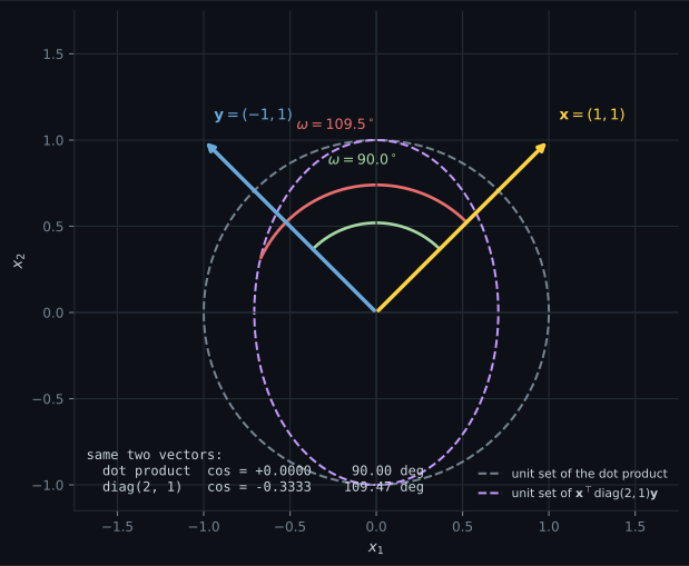
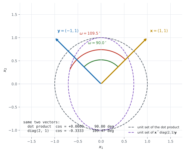
Reading the plot

From the two arcs. The figure draws both angles on the same pair of arrows, which makes the relativity impossible to explain away. Note which object is actually changing: the arrows are fixed and the unit sets differ. Under the dot product the unit set is a circle; under $\mathrm{diag}(2,1)$ it is an ellipse squashed in $x_1$. Both arrows have their $x_1$-component weighted double, and their $x_1$-components have opposite signs, so the weighting tips the inner product from $0$ to $-1$.

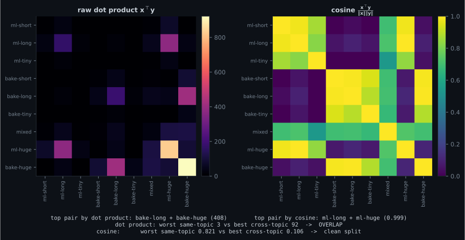
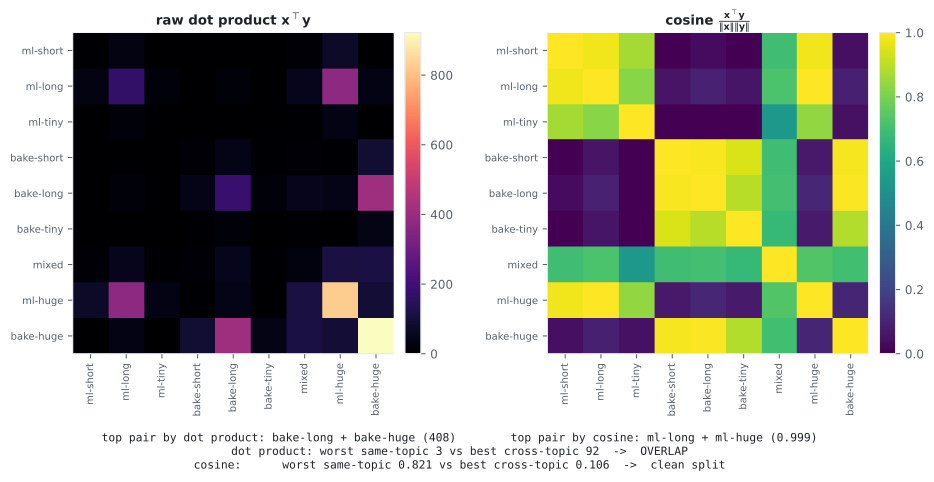
From the heatmaps. This is the sharpest measurement on the page. Nine short documents, three about machine learning, three about baking, three of mixed or extreme length. The dot-product panel is dominated by a bright band on the longest documents: its highest off-diagonal entry is bake-long–bake-huge at $408$, and — the damning number — its worst same-topic score is $3$ while its best cross-topic score is $92$. Ranked by raw dot product, unrelated long documents beat related short ones, and the two groups do not separate at all.

The cosine panel has no such band. Its worst same-topic score is $0.8208$; its best cross-topic score is $0.1057$. A single threshold anywhere between those two values separates the topics perfectly.

One concrete pair makes it vivid. ml-huge and bake-huge share a raw dot product of $92$ — higher than most same-topic pairs — and a cosine of $0.1054$, which is an angle of $83.95°$: almost perpendicular. They look similar to the dot product only because they are both enormous.

And the direct consequence for a retrieval system: asked for the nearest neighbour of ml-tiny, the dot product returns ml-huge (it returns the biggest document that is at all related), while the cosine returns ml-short (the document that is actually most similar in composition).

Pitfalls

arccos of a rounded ratio returns nan

For $\mathbf{y} = c\mathbf{x}$ with $c > 0$ the cosine is mathematically $1$, and in floating point it lands at $1 + 2.2\times10^{-16}$ about half the time. np.arccos(1.0000000000000002) is nan, not $0$. Always np.clip(ratio, -1.0, 1.0) before arccos. This bug is silent until a duplicate row appears in your data, at which point it is silent no longer.

Orthogonality is relative to an inner product

Example 3.7 is the whole warning: $(1,1)$ and $(-1,1)$ are orthogonal under the dot product and meet at $109.47°$ under $\mathrm{diag}(2,1)$. If you whiten your features, decorrelate them, or apply any non-orthogonal transformation, angles change. Two features that were uncorrelated before whitening are generally not perpendicular in the whitened coordinates and vice versa.

Cosine similarity is not a metric

$1 - \cos\omega$ fails the triangle inequality. The angular distance $\omega$ itself is a metric on the unit sphere, and so is $\sqrt{2(1-\cos\omega)}$, which is just the Euclidean distance between the normalised vectors. If you need metric-tree indexing on cosine similarity, normalise and use Euclidean distance — they give the identical ranking.

An orthogonal matrix can be a reflection

$\mathbf{A}^\top\mathbf{A} = \mathbf{I}$ gives $\det(\mathbf{A}) = \pm 1$, and both signs occur. $\mathrm{diag}(1,-1)$ is orthogonal with determinant $-1$. It preserves all lengths and all unsigned angles, and it reverses orientation — so if handedness matters (3-D pose, chirality, mirrored images), checking $\mathbf{A}^\top\mathbf{A} = \mathbf{I}$ is not enough. Check the determinant too. Note also that np.linalg.qr makes no promise about the sign; the $\mathbf{Q}$ it returns is frequently a reflection.

Zero vectors have no angle, but they are orthogonal to everything

Definition 3.7 is stated as $\langle\mathbf{x},\mathbf{y}\rangle = 0$ rather than $\omega = 90°$ precisely so that $\mathbf{0}$ is covered. Code that computes orthogonality via arccos will divide by zero on a zero vector; code that tests the inner product against zero will not.

Compare

quantity	formula	range	scale-free?	is it a metric?
inner product	$\langle\mathbf{x},\mathbf{y}\rangle$	$\mathbb{R}$	no	no (it is a similarity)
cosine similarity	$\dfrac{\langle\mathbf{x},\mathbf{y}\rangle}{\lVert\mathbf{x}\rVert\lVert\mathbf{y}\rVert}$	$[-1,1]$	yes	no
angle $\omega$	$\arccos(\cos\omega)$	$[0,\pi]$	yes	yes, on the unit sphere
$1 - \cos\omega$	—	$[0,2]$	yes	no — fails the triangle inequality
chord distance	$\sqrt{2(1-\cos\omega)}$	$[0,2]$	yes	yes — it is Euclidean distance after normalising

pch.quizTag Check your understanding

1. Why is cosine similarity preferred to the raw dot product for comparing documents or embeddings?

   A It is faster to compute B It is scale-free, so it answers only 'do these point the same way' — the measured heatmaps on this page show the raw dot product's worst same-topic score (3) beaten by its best cross-topic score (92), so the two topic groups do not separate at all C It is bounded, and bounded quantities are always better D The dot product can be negative
   pch.quizShowAnswer

   B — It is scale-free, so it answers only 'do these point the same way' — the measured heatmaps on this page show the raw dot product's worst same-topic score (3) beaten by its best cross-topic score (92), so the two topic groups do not separate at all — The cosine panel separates cleanly: worst same-topic 0.8208 against best cross-topic 0.1057. The concrete failure is that ml-huge and bake-huge share a dot product of 92 while their cosine is 0.1054, an angle of 83.95 degrees.

2. In the measured table, the standard deviation of the cosine between two random vectors in d dimensions tracks which quantity?

   A 1/d B 1/sqrt(d) C log d D It is constant
   pch.quizShowAnswer

   B — 1/sqrt(d) — Measured across d = 2 to d = 10000 the two columns agree to three significant figures. The mean angle stays at 90 degrees throughout — what changes is the spread, from 52 degrees in the plane to 0.56 degrees at d = 10000.

3. Definition 3.7 states orthogonality as the inner product being zero rather than as the angle being ninety degrees. Why does that matter?

   A It does not; the two are equivalent B Because the zero vector has no well-defined angle with anything — the cosine would divide by zero — while its inner product with everything is zero, so the inner-product form correctly makes it orthogonal to everything C Because angles are only defined in two dimensions D Because the cosine can exceed one
   pch.quizShowAnswer

   B — Because the zero vector has no well-defined angle with anything — the cosine would divide by zero — while its inner product with everything is zero, so the inner-product form correctly makes it orthogonal to everything — It is also the practical reason to implement an orthogonality test as a comparison of the inner product against zero rather than via arccos, which would both divide by zero and return nan on a rounded ratio.

4. A matrix satisfies A-transpose A = I. What can you conclude, and what can you not?

   A It is a rotation B It preserves every length and every unsigned angle, and its determinant is plus or minus one — so it may be a reflection and may reverse orientation. det(A) = +1 is the extra condition for a rotation C It is symmetric D Its eigenvalues are all one
   pch.quizShowAnswer

   B — It preserves every length and every unsigned angle, and its determinant is plus or minus one — so it may be a reflection and may reverse orientation. det(A) = +1 is the extra condition for a rotation — diag(1, -1) is orthogonal with determinant -1. Measured across n = 2 to 12, np.linalg.qr returns det(Q) = (-1)^(n-1) deterministically — Householder QR applies n-1 reflections — so in every even dimension its Q is a reflection, which matters whenever handedness does.

🧪 Try It Yourself

Exercise 1 – Angle under an arbitrary inner product

pch.exerciseTag pch.exerciseTitle

Exercise 2 – Make arccos return nan, then fix it

pch.exerciseTag pch.exerciseTitle

Exercise 3 – Reproduce the retrieval failure

pch.exerciseTag pch.exerciseTitle

Exercise 4 – Verify Equations 3.31 and 3.32

pch.exerciseTag pch.exerciseTitle

Exercise 5 – Concentration of measure, measured

pch.exerciseTag pch.exerciseTitle

Recall card

• The cosine of the angle is the inner product divided by both lengths, and Cauchy-Schwarz is what confines it to minus one through one so that arccos applies.
• The angle is unsigned, always between zero and pi, because the inner product is symmetric.
• Orthogonality means the inner product is zero — stated that way rather than as ninety degrees, so that the zero vector is orthogonal to everything.
• Orthogonality is relative to an inner product: the book’s Example 3.7 has one pair at ninety degrees under the dot product and 109.47 degrees under a diagonal reweighting, with cosine exactly minus one third.
• Orthonormal is orthogonal plus unit length, and the second half is what makes coordinates cheap from section 3.5 onwards.
• An orthogonal matrix has A-transpose A equal to the identity, so its inverse is its transpose, and it preserves every length and every angle. Its determinant is plus or minus one, so it may be a reflection.
• Cosine similarity is scale-free and the dot product is not — measured on nine documents, the dot product’s worst same-topic score is beaten by its best cross-topic score, and the cosine separates the two groups cleanly.
• In high dimensions random vectors are nearly perpendicular: the spread of the cosine falls like one over the square root of the dimension, reaching half a degree at ten thousand.

Next: Orthonormal Basis — what orthogonality buys once you build a whole coordinate system out of it.