Tensors and Tensor Operations

A neural network is a pipeline of tensor operations. Nearly every bug in Phase 1 is a shape bug, every speed problem is a dtype or flop-count problem, and both become obvious once you can read a shape and count a multiply. This page is that vocabulary, with the arithmetic and the timings measured rather than asserted.

What you’ll learn

• Rank, shape, size and dtype — and how to compute a tensor’s memory from them.
• The broadcasting rule, tested on six shape pairs including the two that fail.
• Why a matmul costs $2mnk$ flops, and what that predicts when you double $n$ (measured: 7.00× against the theoretical 8).
• Which operations return a view and which copy, verified with np.shares_memory.
• Why converting MNIST to float32 costs exactly 4× the memory.
• A measured surprise: float16 was 314× slower than float32 here, so “half precision to save memory” is not free.

Rank, shape, size, dtype

A tensor is an $n$-dimensional array, and four numbers describe it completely:

Tensor	Rank	Shape	Size	Bytes (float32)
scalar	0	()	1	4
vector	1	(3,)	3	12
matrix	2	(3, 4)	12	48
batch of images	4	(32, 28, 28, 1)	25,088	100,352

Rank is len(shape). Size is the product of the shape. Bytes is $\text{size} \times \text{itemsize}$ — 4 for float32, 8 for float64.

That last row is the shape every image model in Phase 3 consumes: $(\text{batch}, \text{height}, \text{width}, \text{channels})$. Keras calls that axis order channels_last and uses it by default.

diagram Diagram mermaid

  flowchart LR
  A["one image
(28, 28)"] --> B["add a channel axis
(28, 28, 1)"]
  B --> C["stack a batch
(32, 28, 28, 1)"]
  C --> D["flatten for Dense
(32, 784)"]
  D --> E["Dense(128)
(32, 128)"]
  E --> F["Dense(10)
(32, 10)"]
  N["the first axis is the batch axis —
Keras prints it as None because
the model accepts any batch size"] -.-> C

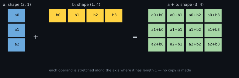
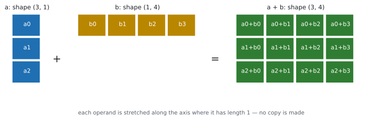
Broadcasting, including where it stops

Adding a bias vector to a matrix of activations needs no loop, because of broadcasting. The rule: align the shapes from the right; each pair of axes must be equal, or one of them must be 1.

figure A (3,1) and a (1,4) add to a (3,4) matplotlib

Each operand is stretched along the axis where its length is 1. No copy is made — the stretch is a striding trick, which is why adding a 4096-element bias to a 4096x4096 matrix costs no extra memory for the bias.

Tested on six pairs:

a	b	result
(3, 4)	(4,)	(3, 4) — one bias per column
(3, 4)	(3, 1)	(3, 4) — one scale per row
(3, 1)	(1, 4)	(3, 4) — both stretch
(32, 28, 28, 1)	(1,)	(32, 28, 28, 1) — a scalar reaches everything
(3, 4)	(3,)	ValueError
(2, 3)	(3, 2)	ValueError

The fifth row is the one that bites. (3, 4) + (3,) reads like “add one number per row”, but right-alignment pairs the 3 against the 4 and neither is 1. What you meant was (3, 1) — written b[:, None] or b.reshape(-1, 1).

Broadcasting does not copy. A 4096×4096 float32 matrix is 67,108,864 bytes; the 4096-element bias added to it is 16,384. Materialising that bias to the matrix’s shape would cost another 67 MB. np.broadcast_to hands you the stretched view with a base of 16,384 bytes — the stretch is bookkeeping, not memory.

Matmul: the operation that dominates the bill

For $\mathbf{A} \in \mathbb{R}^{m \times k}$ and $\mathbf{B} \in \mathbb{R}^{k \times n}$:

$$(\mathbf{A}\mathbf{B})_{ij} = \sum_{p=1}^{k} A_{ip} B_{pj}$$

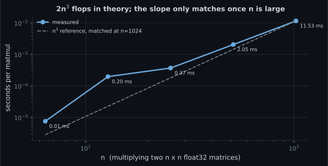
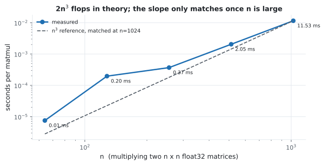
Each of the $mn$ output entries costs $k$ multiplies and $k-1$ adds, so the total is $mn(2k-1) \approx 2mnk$ flops. For square matrices that is $2n^3$, so doubling $n$ multiplies the work by 8.

figure Measured matmul time against the n³ prediction matplotlib

Between 64 and 256 the measurement is flatter than n cubed because fixed overheads and cache effects dominate — at n=128 the matmul took 0.29 ms against 0.34 ms at n=256, which is not a typo. From 512 upward the slope matches: 512 to 1024 multiplied the time by 7.00 against a predicted 8.

n	flops	seconds	GFLOP/s
64	524,288	0.000009	61.25
128	4,194,304	0.000139	30.27
256	33,554,432	0.000354	94.79
512	268,435,456	0.001542	174.09
1024	2,147,483,648	0.010800	198.84

Two lessons. The asymptotic rule only applies asymptotically — below a few hundred elements per side you are timing overhead, not arithmetic. And throughput improves with size: 61 GFLOP/s at n=64 against 199 at n=1024, because large matrices amortise the cost of moving data into cache. That is the real reason mini-batching exists — 32 images through one matmul beats 32 separate matmuls even though the flop count is identical.

You can price a forward pass the same way. A 784→128→10 MLP on a batch of 32:

$$2 \cdot 32 \cdot 784 \cdot 128 \;+\; 2 \cdot 32 \cdot 128 \cdot 10 = 6{,}504{,}448 \text{ flops}$$

That is 203,264 flops per image, and the first layer is 98.7% of it.

Views, copies and strides

reshape and transpose do not move data — they change how the same bytes are read. That is fast, and it means an accidental shared view is a bug waiting to happen:

views_and_copies.py

import numpy as np
 
a = np.arange(12, dtype="float32")
b = a.reshape(3, 4)        # a view
c = b.T                    # also a view
d = b.copy()               # a real copy
 
print(np.shares_memory(a, b))    # True
print(np.shares_memory(a, c))    # True
print(np.shares_memory(a, d))    # False
 
b[0, 0] = 99.0
print(a[0], d[0, 0])             # 99.0 0.0  -- writing through the view changed a
print(b.strides, c.strides)      # (16, 4) (4, 16)  -- transpose swaps strides

A float32 row of 4 elements advances 16 bytes per row and 4 per column, so b.strides is (16, 4). Transposing swaps them to (4, 16) without touching a byte — which is why c.flags['C_CONTIGUOUS'] is False, and why some later operation on a transpose may quietly materialise a contiguous copy.

dtype is a decision, not a detail

figure Memory behaves as expected; speed does not matplotlib

float16 halves the memory and, on this CPU, took hundreds of times longer for the same matmul — there is no native half-precision kernel here, so the work is emulated. float64 costs twice float32's memory and roughly twice its time, which is the trade you would predict.

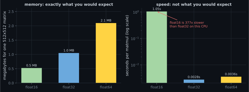
dtype	bytes for 2048×2048	matmul time
float16	8,388,608	135.92 s
float32	16,777,216	0.0774 s
float64	33,554,432	0.1510 s

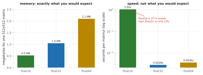
At $n = 2048$ the float16 penalty was a factor of 1,756. The figure repeats the experiment at $n = 512$, where the same effect measures 314× — the ratio depends on size, but the direction never changes on a CPU with no half-precision hardware. The lesson is not “never use float16”: it is that half precision pays on hardware built for it and costs dearly on hardware without it. Phase 8 measures mixed precision properly.

float32 is the deep-learning default because it halves float64’s memory and bandwidth while keeping enough precision for gradients. It does run out of integers, though:

float32_limit.py

import numpy as np
 
total = np.float32(16_777_210.0)
for step in range(1, 9):
    total = total + np.float32(1.0)
    print(step, total)
# 1 16777211.0 ... 5 16777215.0   6 16777216.0   7 16777216.0   8 16777216.0

With 23 mantissa bits, $2^{24} = 16{,}777{,}216$ is the last integer float32 represents exactly. Adding 1.0 past it does nothing — silently. The same loop in float64 reaches 16,777,218, which is why counters and step numbers live in int64.

Shape errors, and how Keras reports them

A 784-input model given the wrong shape fails in three distinguishable ways:

Input	Result
(5, 784)	works — output (5, 10)
(5, 28, 28)	ValueError from Sequential.call() — rank mismatch, caught early
(5, 783)	InvalidArgumentError at graph execution — the matmul itself refused

The middle case is the friendly one: Keras compares ranks before doing any work. The last reaches the kernel, which is why its message is longer and less obvious. Both mean the same thing — what you passed does not match what the first layer declared.

One dataset, four shapes

MNIST as it arrives, and as each model wants it:

Representation	Shape	dtype	Bytes
raw dataset	(60000, 28, 28)	uint8	47,040,000
flattened and scaled	(60000, 784)	float32	188,160,000
with a channel axis	(60000, 28, 28, 1)	float32	188,160,000
labels, one-hot	(60000, 10)	float64	4,800,000

Dividing by 255 is not free: it converts uint8 to float32 and multiplies the memory by 4. On a dataset this size that is invisible; on a large image corpus it is exactly why tf.data streams from disk and scales inside the pipeline instead of up front.

See it move

The first sketch is the shape algebra: watch each axis get checked, and see which pairs are legal.

sketch Broadcasting, one axis at a time p5.js Pause Restart

Two shapes are aligned from the right, each axis pair is checked against the rule, and the result shape is assembled. Click to cycle through compatible and incompatible pairs.

The second sketch contrasts the two operations people conflate: reshaping rearranges the same numbers, while broadcasting re-reads a smaller tensor for every row.

sketch Reshape vs. broadcast p5.js Pause Restart

Left: the six cells of a (3,2) grid continuously re-flow into a (2,3) grid and back -- same values, same order, just a new shape. Right: the vector's virtual copy sweeps down through every row it's broadcast onto.

Chollet’s uncrumpled paper ball

Think of the input as two crumpled sheets of coloured paper balled together. Training is finding a sequence of simple geometric moves — translations (+), rotations and scalings (@), and non-linear folds (activations) — that uncrumples the ball until the two colours separate. Every one of those moves is a tensor operation from this page.

Pitfalls

Reading (3, 4) + (3,) as “one value per row”. Right-alignment pairs 3 with 4 and raises. Use b[:, None] to get (3, 1).

Forgetting the batch axis. A single 784-vector must be (1, 784), not (784,). Keras prints the model’s input as (None, 784); that None is the batch axis and it is never optional.

Writing through a view by accident. b = a.reshape(3, 4) shares memory, so b[0, 0] = 99 changes a. Call .copy() when you need independence — and not when you do not, because on large arrays it is the expensive line.

Choosing float16 to save memory on a CPU. Measured here: 314× slower at n=512, 1,756× at n=2048. Half precision belongs on hardware built for it.

Accumulating counters in float32. Past $2^{24}$, total += 1.0 silently stops increasing.

Assuming a transpose stays free. Transposing is free; the next operation may materialise a contiguous copy of it.

Recap

• Rank is len(shape), size is the product of the shape, bytes is $\text{size} \times \text{itemsize}$.
• Broadcasting aligns from the right and needs each axis pair equal or containing a 1. Six pairs tested, two failed, and the stretch never copies.
• Matmul is $\approx 2mnk$ flops, so doubling a square side costs 8× — measured 7.00× from 512 to 1024, with throughput climbing from 61 to 199 GFLOP/s because bigger matmuls use cache better. That is why mini-batching helps.
• A 784→128→10 forward pass is 203,264 flops per image, 98.7% in the first layer.
• reshape and .T return views sharing memory; only .copy() does not.
• float32 is the default: half of float64’s memory, and hundreds of times faster than float16 on this CPU. It stops counting integers exactly at $2^{24}$.
• Scaling MNIST to float32 multiplies its memory by exactly 4.

pch.quizTag pch.quizDefaultTitle

1. You have activations of shape (32, 128) and a bias of shape (128,). What does adding them produce?

   A An error, because the ranks differ B Shape (32, 128) — right-alignment pairs 128 with 128 and the missing axis counts as 1, so the bias is stretched across all 32 rows without being copied C Shape (32, 128, 128) D Shape (160,)
   pch.quizShowAnswer

   B — Shape (32, 128) — right-alignment pairs 128 with 128 and the missing axis counts as 1, so the bias is stretched across all 32 rows without being copied — This is exactly what a Dense layer does internally. Contrast (3, 4) + (3,), which fails because there the 3 lines up against the 4.

2. A 512x512 matmul takes 1.5 ms. Roughly how long should 1024x1024 take?

   A About 3 ms — twice the size, twice the work B About 12 ms — the flop count is 2n³, so doubling n multiplies the work by 8; measured here it was 7.00x C About 6 ms D The same, because the hardware parallelises it
   pch.quizShowAnswer

   B — About 12 ms — the flop count is 2n³, so doubling n multiplies the work by 8; measured here it was 7.00x — Measured: 1.542 ms at n=512 and 10.800 ms at n=1024, a factor of 7.00. It came in under 8 because the larger matmul reached higher throughput — 199 GFLOP/s against 174.

3. b = a.reshape(3, 4), then b[0, 0] = 99. What happened to a?

   A Nothing — reshape returns a new array B a[0] is now 99.0, because reshape returned a view sharing the same memory; only .copy() gives independence C a raises an error on next access D It depends on the dtype
   pch.quizShowAnswer

   B — a[0] is now 99.0, because reshape returned a view sharing the same memory; only .copy() gives independence — np.shares_memory(a, b) is True. The same holds for a transpose, which merely swaps strides from (16, 4) to (4, 16) without moving a byte.

4. You switch a CPU run from float32 to float16 to halve memory. What does the measurement here predict?

   A Roughly 2x faster, since there is half as much data to move B Dramatically slower — 314x at n=512 and 1,756x at n=2048 on this CPU, because there is no native half-precision kernel and the work is emulated C Identical speed, half the memory D A crash
   pch.quizShowAnswer

   B — Dramatically slower — 314x at n=512 and 1,756x at n=2048 on this CPU, because there is no native half-precision kernel and the work is emulated — Memory halved exactly as expected; only the time was surprising. Half precision is a win on hardware with tensor cores and a serious loss without them.

5. Why does mini-batching speed up training when it does not change the flop count?

   A It reduces the number of gradient updates B One large matmul reaches far higher throughput than many small ones — 199 GFLOP/s at n=1024 against 61 at n=64 — because large operations amortise the cost of moving data into cache C Because broadcasting is free D It lowers the precision required
   pch.quizShowAnswer

   B — One large matmul reaches far higher throughput than many small ones — 199 GFLOP/s at n=1024 against 61 at n=64 — because large operations amortise the cost of moving data into cache — The arithmetic is identical; the memory traffic per flop is not. It is also why the measured curve is flatter than n³ at small sizes — there you are timing overhead rather than multiplication.

Next

You can now read a shape, price a matmul and predict a memory footprint. Continue to Introduction to Neural Networks (The Perceptron), where these tensors become one neuron’s weighted sum and the shapes start to mean something.

🧪 Try It Yourself

Exercise 1 – Read a tensor’s four properties

pch.exerciseTag pch.exerciseTitle

Exercise 2 – Predict which shapes broadcast

pch.exerciseTag pch.exerciseTitle

Exercise 3 – Tell a view from a copy

pch.exerciseTag pch.exerciseTitle

Exercise 4 – Count the flops in a forward pass

pch.exerciseTag pch.exerciseTitle

Exercise 5 – Watch float32 run out of integers

pch.exerciseTag pch.exerciseTitle

Exercise 6 – The four shapes of one dataset

pch.exerciseTag pch.exerciseTitle