Hyperparameter Tuning with KerasTuner

Hyperparameter search has one honest measurement: best result found per unit of compute spent. Any comparison that lets one strategy train for longer than another is measuring the budget, not the strategy.

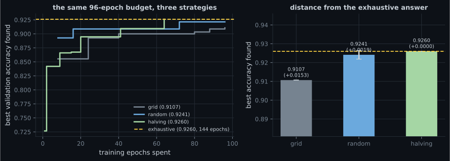
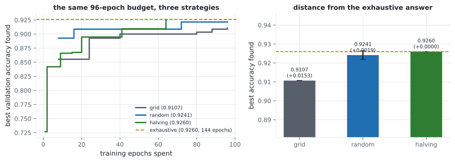
Three strategies over the same 18-configuration space, each given exactly 96 training epochs:

Strategy	Best found	Epochs spent	Gap to the exhaustive answer
Grid	0.9107	96	+0.0153
Random	0.9241 ± 0.0023	96	+0.0019
Successive halving	0.9260	64	+0.0000
Exhaustive	0.9260	144	—

Successive halving found the exact best configuration — units 128, learning rate 3e-3, dropout 0.3 — using 44% of what an exhaustive search needed, and it stopped early with budget to spare.

What you’ll learn

Why grid search is the weakest of the three despite sounding the most thorough.
How successive halving spends its budget, rung by rung.
The assumption it depends on — measured here at r = 0.9126 — and what happens when that assumption fails.
Why one hyperparameter dominated this search space, and how to find that out cheaply.

The three strategies

Random search, in full

for _ in range(trials):
    config = {name: rng.choice(values) for name, values in space.items()}
    score = train(**config, epochs=FULL_EPOCHS)
    best = max(best, score)

Successive halving, in full

survivors = list(space)
for epochs in (1, 2, 5):                     # each rung trains longer
    scored = [(train(**c, epochs=epochs), c) for c in survivors]
    scored.sort(reverse=True, key=lambda pair: pair[0])
    survivors = [c for _, c in scored[:len(scored) // 2]]   # keep the best half

The idea behind halving is that a bad configuration usually looks bad quickly. Instead of giving every candidate a full run, give them all a cheap one, discard the worst half, and reinvest the saved budget in the survivors.

figure 18 configurations, 96-epoch budget each, 5 seeds for the randomised strategies matplotlib

Halving's curve is the interesting one: it climbs in steps as each rung promotes its survivors, and it reaches the exhaustive answer with a third of its budget unspent. Grid search is the flat line — it works through the space in a fixed order and simply ran out of budget before reaching the good corner, which is a property of the ordering rather than of the space.

Why grid search loses

Grid search is exhaustive-in-principle and arbitrary-in-practice. Given a partial budget it evaluates a prefix of the space in whatever order the loops happen to nest — so its result depends on which hyperparameter you put in the outer loop.

That is why it finished 0.0153 behind. It is not that grid search is a bad algorithm; it is that “grid search with an insufficient budget” is really “arbitrary subset search”, and nobody chooses the subset deliberately.

Random search avoids exactly that failure. Its 0.9241 ± 0.0023 across five seeds is close to optimal, and it has no ordering bias to exploit or fall foul of.

What halving actually does

figure One run of successive halving, and the assumption underneath it matplotlib

The left panel shows the budget being concentrated: 18 cheap runs, then 9, then 4. The spread within rung 0 is enormous — 0.8673 down to 0.3753 — which is exactly the condition that makes early elimination safe, since the bottom half is obviously hopeless after a single epoch. The right panel is the assumption stated as a measurement: r = 0.9126 between a one-epoch score and an eight-epoch score.

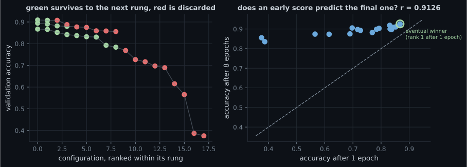
Rung	Configurations	Epochs each	Best	Worst	Kept
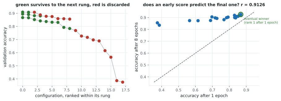
0	18	1	0.8673	0.3753	9
1	9	2	0.8947	0.8560	4
2	4	5	0.9093	0.8880	2

Notice how the worst score rises at every rung — 0.3753, then 0.8560, then 0.8880. That is the method working: each round removes the candidates that were obviously failing, and the survivors become progressively harder to separate.

The assumption, and when it breaks

Halving assumes early performance ranks configurations roughly the way final performance does. Here it did: the correlation between a 1-epoch score and an 8-epoch score was 0.9126, and the eventual winner was already ranked #1 of 18 after a single epoch.

That is a property of this search space, not a law. It fails in recognisable situations:

A low learning rate that eventually wins. It looks terrible after one epoch and is eliminated before it can demonstrate anything.
Heavy regularisation. Dropout and weight decay cost training accuracy early and pay it back late.
Warm-up schedules, which are designed to look bad at the start.

When the assumption fails, halving does not degrade gracefully — it confidently discards the best option in the first rung and then spends the whole remaining budget on the survivors. The cheap diagnostic is exactly the right-hand panel above: score the space at both lengths once, and look at the correlation before trusting the method.

diagram Diagram mermaid

  flowchart TD
  S["18 configurations"] --> R0["rung 0: 1 epoch each
0.3753 to 0.8673"]
  R0 -->|"keep the best 9"| R1["rung 1: 2 epochs each
0.8560 to 0.8947"]
  R1 -->|"keep the best 4"| R2["rung 2: 5 epochs each
0.8880 to 0.9093"]
  R2 -->|"keep the best 2"| F["full run for the leader
0.9260"]
  R0 -.->|"assumes early rank ~ final rank
r = 0.9126 here"| A["if that fails, the winner
is discarded in rung 0"]

The search space itself

figure Every configuration trained for the full 8 epochs matplotlib

The right panel is worth more than the search results. Learning rate separates the space almost by itself — the mean accuracy climbs monotonically across the three values while the error bars, which cover every combination of units and dropout, stay narrow. Units and dropout barely matter here by comparison, which means most of the search budget was spent distinguishing configurations that were never going to differ much.

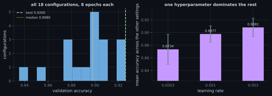
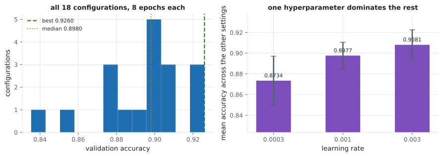
The full space spans 0.8353 to 0.9260 — a range of 0.0907. If that range had been 0.005, no search strategy would have been worth running at all, and the correct decision would have been to spend the compute on training instead.

Measure the spread before optimising the search. A cheap random sample of six configurations tells you whether the space is worth searching, and that is the question that determines whether any of this matters.

The library version

For reference, the same two algorithms through KerasTuner’s API. This is not executed on this page:

KerasTuner (shown, not run here)

import keras_tuner as kt
 
def build(hp):
    units = hp.Choice("units", [32, 64, 128])
    model = keras.Sequential([
        keras.layers.Input((784,)),
        keras.layers.Dense(units, activation="relu"),
        keras.layers.Dropout(hp.Choice("dropout", [0.0, 0.3])),
        keras.layers.Dense(units, activation="relu"),
        keras.layers.Dense(10, activation="softmax"),
    ])
    model.compile(keras.optimizers.Adam(hp.Choice("rate", [3e-4, 1e-3, 3e-3])),
                  "sparse_categorical_crossentropy", metrics=["accuracy"])
    return model
 
tuner = kt.Hyperband(build, objective="val_accuracy", max_epochs=8, factor=2)
tuner.search(x_train, y_train, validation_data=(x_test, y_test))

kt.Hyperband is successive halving run several times with different starting rung lengths, which hedges against exactly the assumption failure described above. kt.RandomSearch is the random strategy, and kt.BayesianOptimization fits a model of the objective — worth it when a single trial is expensive enough that the fitting cost disappears next to it.

sketch Where the budget goes p5.js

Drag the two sliders to change how many configurations start and how aggressively each rung prunes. The bars show the epochs spent at each rung.

sketch The measured table, ranked p5.js

Click a column to rank every row by it. The bars are that column's values and the highest and lowest are computed from the numbers, not written in.

Pitfalls

Comparing strategies on different budgets. Exhaustive “won” on 144 epochs; on 96 it would not have finished.
Grid search with a partial budget. It becomes an arbitrary subset chosen by loop order — 0.0153 behind here.
Trusting halving without checking the rank correlation. It was 0.9126 here; when it is low, the method eliminates the winner in rung 0.
Searching a space that does not vary. Measure the spread first — 0.0907 here justified the search; 0.005 would not have.
Reporting a single seed for a randomised strategy. Random search varied by 0.0023 across five seeds.
Tuning everything at once. Learning rate dominated; units and dropout barely separated the space.
Forgetting that the validation set is being optimised against. Search enough configurations and the best one is partly fitted to the validation split.

Recap

Compare search strategies at equal compute, or you are comparing budgets.
Successive halving found the exact best configuration in 64 epochs; exhaustive needed 144.
Grid search with a partial budget is an arbitrary subset — it finished 0.0153 short.
Random search reached 0.9241 ± 0.0023 and has no ordering bias.
Halving depends on early rank predicting final rank; measured at r = 0.9126, with the winner already first after one epoch.
Learning rate dominated this space, so most of the budget separated configurations that differed little.

Tuning finds a better model; the remaining pages are about running one. First, spreading a single training job across devices: Distributed Training with tf.distribute.

pch.quizTag pch.quizDefaultTitle

Successive halving found the best configuration in 64 epochs while grid search missed it with 96. What went wrong for grid search?

pch.quizShowAnswer

B — With a partial budget it evaluates a prefix of the space in whatever order the loops nest, so it is really an arbitrary subset search — and nobody chooses that subset deliberately — Given the full 144-epoch budget grid search would find the same answer as exhaustive search. The failure is specific to being cut short.
What assumption does successive halving depend on, and how was it checked here?

pch.quizShowAnswer

B — That early performance ranks configurations roughly the way final performance does — checked by correlating 1-epoch and 8-epoch scores, which gave r = 0.9126 — The eventual winner was already ranked first of 18 after a single epoch, which is why the method worked so well on this space.
In which situation would successive halving be most likely to discard the best configuration?

pch.quizShowAnswer

B — When a configuration is designed to look bad early — a low learning rate, heavy regularisation, or a warm-up schedule that pays off only later — It does not degrade gracefully: the winner is eliminated in rung 0 and the whole remaining budget goes to the survivors.
The worst score per rung rose from 0.3753 to 0.8560 to 0.8880. What does that pattern show?

pch.quizShowAnswer

B — The method is working — each rung removes the obviously failing candidates, so the survivors become progressively harder to distinguish — The large spread in rung 0 is exactly the condition that makes cheap early elimination safe.
Mean accuracy rose monotonically with learning rate while units and dropout barely mattered. What follows for the search?

pch.quizShowAnswer

B — Most of the budget was spent separating configurations that were never going to differ much — knowing which hyperparameter dominates lets you spend the next search where it counts — A cheap sample of a handful of configurations reveals both the spread of the space and which axis is doing the work, before committing to a full search.

🧪 Try It Yourself

pch.coffeeTagline

pch.coffeeCta

pch.feedbackHeading

pch.feedbackSubheading