
Partial Differentiation and Gradients
Everything on the previous page had one input. Real functions do not: a loss depends on every weight in the network at once. The generalisation is almost anticlimactic — vary one variable and hold the others fixed — and the only genuinely new thing is what you do with the answers once you have of them.
You collect them into a vector. The book collects them into a row vector, and that choice is not cosmetic: it is what lets §5.3 write the multivariate chain rule as a plain matrix product with no transposes to remember.
What you’ll learn
Section titled “What you’ll learn”- Definition 5.5: the partial derivative, which is Definition 5.2 with the other variables frozen.
- Equation 5.40: the gradient as a row vector, and the book’s two reasons for the row convention.
- Three claims about the gradient, each measured: it is the direction of steepest ascent, its norm is that steepest rate, and it is perpendicular to the level set.
- §5.2.1: the product, sum and chain rules survive — with one warning, since matrix multiplication does not commute.
- §5.2.2 and Equation 5.53: the multivariate chain rule, as a matrix product.
- Where the difference quotient’s round-off floor lands in several dimensions, and why gradient checking needs a relative tolerance.
Intuition: climbing a hill in fog
Section titled “Intuition: climbing a hill in fog”You are on a hillside and cannot see. You can feel the slope under your feet in the two compass directions — north–south and east–west — and that is all.
Those two numbers are the partial derivatives. And they are enough: the direction of steepest ascent is not “whichever of the two is bigger”, it is the combination of them, and the vector points exactly that way. Its length is how steep the hill is in that best direction. Walk perpendicular to it and your altitude does not change — you are following a contour.
None of that is obvious from the definition, and all of it is checkable.
  flowchart TD
  PD["partial derivative
∂f/∂xᵢ = lim (f(…xᵢ+h…) − f(x))/h
Def 5.5 — freeze the others"]
  PD --> G["gradient / Jacobian
∇ₓf = [∂f/∂x₁ … ∂f/∂xₙ] ∈ ℝ¹ˣⁿ
Eq 5.40 — a ROW"]
  G --> W1["why a row, reason 1:
it generalises to f: ℝⁿ→ℝᵐ
with no shape change (§5.3)"]
  G --> W2["why a row, reason 2:
the chain rule becomes a
plain matrix product"]
  G --> C1["steepest ascent:
argmax_d ∇f·d = ∇f/‖∇f‖"]
  G --> C2["steepest rate:
max_d ∇f·d = ‖∇f‖"]
  G --> C3["⊥ to the level set:
∇f · (contour tangent) = 0"]
  G --> CR["chain rule §5.2.2
df/d(s,t) = (∂f/∂x)(∂x/∂(s,t))
Eq 5.53 — (1×2)(2×2)"]
  CR --> BP["§5.6 backpropagation
is this, n layers deep"]
  C1 --> GD["Ch 7: gradient descent
steps along −∇f"]
The math
Section titled “The math”The partial derivative
Section titled “The partial derivative”Every partial derivative is an ordinary scalar derivative — the book’s own margin note says so — so §5.1’s rules apply unchanged to each one. Nothing new is needed to compute them.
Why the gradient is a row
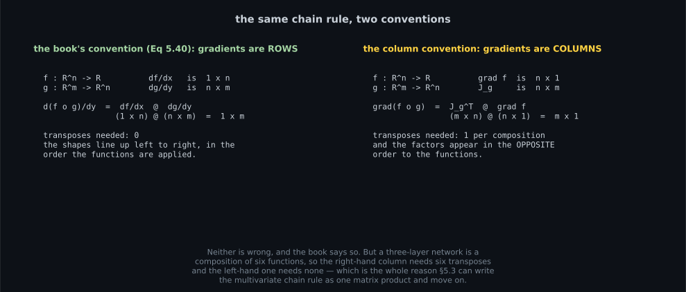
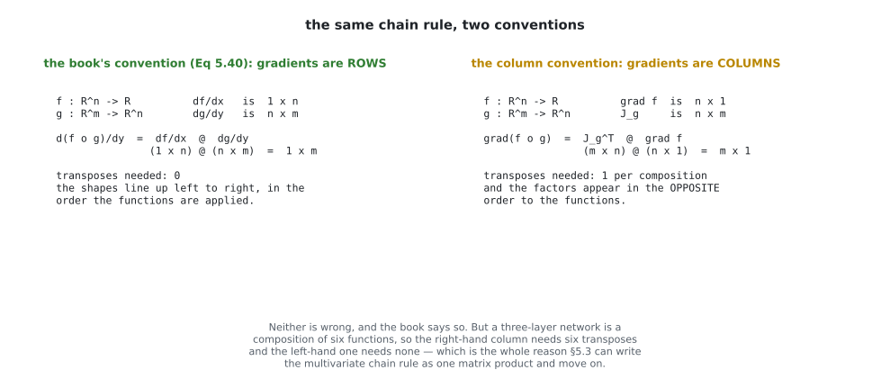
Section titled “Why the gradient is a row”That second reason is the practical one. With the row convention, composing with gives
The shapes chain left to right in the order the functions are applied, and there is nothing to transpose. With the column convention the same composition is — one transpose, and the factors in the opposite order to the functions. Neither is wrong; one of them costs a transpose per layer, and a network is a composition of many layers.
The three claims
Section titled “The three claims”Nothing in Definition 5.5 mentions steepness or perpendicularity. Both follow from one identity. For a unit direction , the directional derivative is
using §3.4’s definition of the angle. That single line settles all three:
| claim | why |
|---|---|
| the gradient points in the direction of steepest ascent | is largest at , i.e. parallel to |
| the steepest rate equals | at , |
| the gradient is perpendicular to the level set | along a contour does not change, so , so |
The measurements below check each one, because a chain of three “so”s is exactly where a sign error hides.
The rules, with a warning
Section titled “The rules, with a warning”§5.2.1 states that the sum, product and chain rules all still apply. Then it adds the warning that matters:
However, when we compute derivatives with respect to vectors we need to pay attention: our gradients now involve vectors and matrices, and matrix multiplication is not commutative, i.e. the order matters.
The multivariate chain rule
Section titled “The multivariate chain rule”For with and :
and if , depend on two variables, the same rule gives Equations 5.51 and 5.52, which assemble into
Worked example by hand
Section titled “Worked example by hand”Example 5.6 — one inner function, two partials
Section titled “Example 5.6 — one inner function, two partials”. Both partials come from one application of the chain rule to the same inner function :
At : , so
Both verified against a central-difference Jacobian to .
Example 5.7 — the gradient
Section titled “Example 5.7 — the gradient”. Differentiating with respect to each variable in turn, treating the other as a constant:
At this is , so — a –– triangle, which makes the checks below easy to read.
Notice that neither partial derivative is a function of its own variable alone. depends on . That is why the gradient has to be a vector rather than a pair of independent slopes, and it is the whole reason optimising one coordinate at a time does not work.
Example 5.8 — the chain rule along a curve
Section titled “Example 5.8 — the chain rule along a curve”with , :
The factored form is worth keeping: exactly when or , so at every multiple of . And since always, the sign of the derivative is the opposite of the sign of — the function decreases on and increases on .
The three claims, checked
Section titled “The three claims, checked”import numpy as np
# The book's Example 5.7.
f = lambda x, y: x ** 2 * y + x * y ** 3
fx = lambda x, y: 2 * x * y + y ** 3
fy = lambda x, y: x ** 2 + 3 * x * y ** 2
x0, y0 = 1.0, 1.0
grad = np.array([fx(x0, y0), fy(x0, y0)]) # Eq 5.45: a 1 x 2 row
gn = float(np.linalg.norm(grad))
print("Eq 5.45 grad f =", grad, " shape (1, 2) as a row")
print(" |grad f| =", gn)
print()
# CLAIM 1 and 2: sweep every direction and see which wins, and by how much.
th = np.linspace(0, 2 * np.pi, 100001)[:-1]
rate = grad[0] * np.cos(th) + grad[1] * np.sin(th)
i = int(np.argmax(rate))
print("claim 1: the steepest direction is the gradient's own direction")
print(f" gradient angle {np.degrees(np.arctan2(grad[1], grad[0])):.6f} deg")
print(f" sampled argmax {np.degrees(th[i]):.6f} deg")
print("claim 2: the steepest rate equals |grad f|")
print(f" sampled max {rate[i]:.9f}")
print(f" |grad f| {gn:.9f}")
print(f" no direction beat it: {bool(np.all(rate <= gn + 1e-12))}")
print()
# CLAIM 3: perpendicular to the level set. The contour tangent is the gradient
# rotated by 90 degrees, so the inner product must vanish -- and stepping along
# it must leave f almost unchanged.
tangent = np.array([-grad[1], grad[0]]) / gn
print("claim 3: perpendicular to the level set")
print(f" grad . tangent = {float(grad @ tangent):.1e}")
step = 1e-3
along_t = abs(f(x0 + step * tangent[0], y0 + step * tangent[1]) - f(x0, y0))
along_g = abs(f(x0 + step * grad[0] / gn, y0 + step * grad[1] / gn) - f(x0, y0))
print(f" |df| stepping {step} along the tangent: {along_t:.3e}")
print(f" |df| stepping {step} along the gradient: {along_g:.3e}")
print(f" ratio: {along_g / along_t:.0f}x")Eq 5.45 grad f = [3. 4.] shape (1, 2) as a row
|grad f| = 5.0
claim 1: the steepest direction is the gradient's own direction
gradient angle 53.130102 deg
sampled argmax 53.128800 deg
claim 2: the steepest rate equals |grad f|
sampled max 4.999999999
|grad f| 5.000000000
no direction beat it: True
claim 3: perpendicular to the level set
grad . tangent = -4.4e-16
|df| stepping 0.001 along the tangent: 6.803e-07
|df| stepping 0.001 along the gradient: 5.005e-03
ratio: 7357xSee it move
Section titled “See it move”Two limits, one row vector, then the three claims checked in turn. The frame to stop on is the difference-quotient table: the central difference is exact at h = 1 here, because the slice is quadratic, and then round-off makes smaller h worse.
The second derivative of exp(−r²/2) in x is (x²−1)f, which is exactly zero at x = 1 — one of the points evaluated here. The leading forward-difference error is (h/2)f'', so at that point the forward difference is accidentally second order, and the lab says so.
From scratch
Section titled “From scratch”import numpy as np
def numeric_gradient(f, x, h=1e-6):
"""Definition 5.5, one coordinate at a time, centrally. Returns a 1 x n row."""
x = np.asarray(x, dtype=float)
g = np.zeros((1, x.size))
for i in range(x.size):
e = np.zeros_like(x)
e[i] = h
g[0, i] = (f(x + e) - f(x - e)) / (2 * h)
return g
def analytic_gradient(x):
"""Example 5.7, Eq 5.45."""
x1, x2 = x
return np.array([[2 * x1 * x2 + x2 ** 3, x1 ** 2 + 3 * x1 * x2 ** 2]])
f = lambda v: v[0] ** 2 * v[1] + v[0] * v[1] ** 3
print(f"{'point':>16} {'analytic':>26} {'numeric':>26} {'rel err':>9}")
for pt in ([1.0, 1.0], [0.5, -1.5], [2.0, 0.3], [-1.0, 2.0], [0.0, 0.0]):
a = analytic_gradient(pt)
n = numeric_gradient(f, pt)
scale = max(float(np.abs(a).max()), 1e-12)
print(f"{str(pt):>16} {str(np.round(a[0], 6)):>26} {str(np.round(n[0], 6)):>26}"
f" {float(np.abs(a - n).max()) / scale:>9.1e}")
print()
print("shape of the gradient:", analytic_gradient([1.0, 1.0]).shape, "-- a ROW, Eq 5.40")
print()
# The multivariate chain rule, Eq 5.53, as a matrix product.
# f(x1, x2) = x1^2 + 2 x2 with x1 = sin t, x2 = cos t (Example 5.8)
t = 0.7
df_dx = np.array([[2 * np.sin(t), 2.0]]) # 1 x 2
dx_dt = np.array([[np.cos(t)], [-np.sin(t)]]) # 2 x 1
chain = float((df_dx @ dx_dt).item())
closed = 2 * np.sin(t) * (np.cos(t) - 1) # Eq 5.50c
h = 1e-6
g = lambda tt: np.sin(tt) ** 2 + 2 * np.cos(tt)
numeric = (g(t + h) - g(t - h)) / (2 * h)
print("Example 5.8 at t = 0.7")
print(f" (df/dx)(dx/dt), a (1x2)(2x1) product : {chain:.12f}")
print(f" 2 sin t (cos t - 1), Eq 5.50c : {closed:.12f}")
print(f" central difference in t : {numeric:.12f}")
print(f" largest gap : {max(abs(chain-closed), abs(chain-numeric)):.1e}") point analytic numeric rel err
[1.0, 1.0] [3. 4.] [3. 4.] 3.4e-11
[0.5, -1.5] [-4.875 3.625] [-4.875 3.625] 1.0e-10
[2.0, 0.3] [1.227 4.54 ] [1.227 4.54 ] 1.3e-11
[-1.0, 2.0] [ 4. -11.] [ 4. -11.] 5.9e-11
[0.0, 0.0] [0. 0.] [0. 0.] 0.0e+00
shape of the gradient: (1, 2) -- a ROW, Eq 5.40
Example 5.8 at t = 0.7
(df/dx)(dx/dt), a (1x2)(2x1) product : -0.302985644487
2 sin t (cos t - 1), Eq 5.50c : -0.302985644487
central difference in t : -0.302985644463
largest gap : 2.4e-11Three things worth noting.
The shape is (1, 2) — a row. Writing np.array([fx, fy]) gives shape (2,),
which NumPy will happily broadcast in ways that hide a transpose error until the
dimensions stop being equal.
The [0.0, 0.0] row has relative error exactly 0.0e+00, because both partials
are exactly zero there — that is a critical point of Example 5.7, and it is a
saddle, not an optimum.
And the chain rule row is the point of Equation 5.53: the answer comes out of a matrix product, agrees with the hand-factored closed form to every printed digit, and agrees with a direct numerical derivative in to . Three routes, one answer.
One detail in that code is a real trap. float(df_dx @ dx_dt) raises a
TypeError on recent NumPy, because the product is a array rather than a
scalar — the shapes chained correctly and that is exactly why. Use .item().
On real data
Section titled “On real data”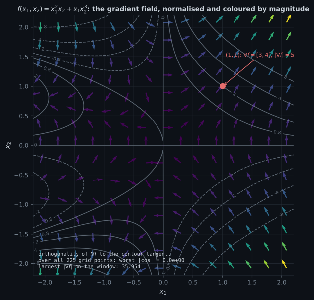
Reading the plot
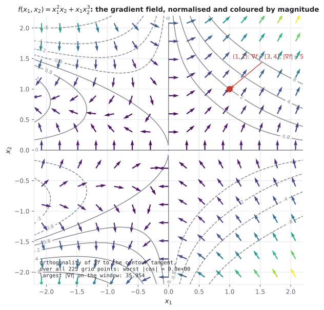
Section titled “Reading the plot”From the gradient field. The reported inner product is 0.0e+00 at all 225
grid points, and it is worth being precise about why. The tangent is constructed
as , so the inner product is
— the same two
products subtracted, which cancels bit-for-bit. Normalise the tangent first, as the
exercises below do, and the same quantity comes back as
instead: the division introduces rounding that the unnormalised form never had.
So that zero is a check on the construction, not on the geometry. The geometric content is that this construction is the contour direction — which the picture shows by the arrows meeting the grey curves squarely, and which the exercises measure by stepping along it.
The step comparison is the geometric check. Moving along the contour tangent changes by ; moving the same distance along the gradient changes it by — 7357 times more. Across four points the ratio runs from to .
The colouring carries the other lesson. Where the contours bunch, the arrows are long; where the surface is flat they nearly vanish. Gradient magnitude is inversely related to contour spacing, which is why gradient descent naturally takes big steps on steep ground and small ones near an optimum — and why it stalls completely on a plateau.
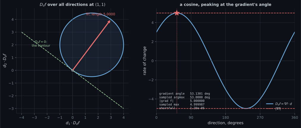
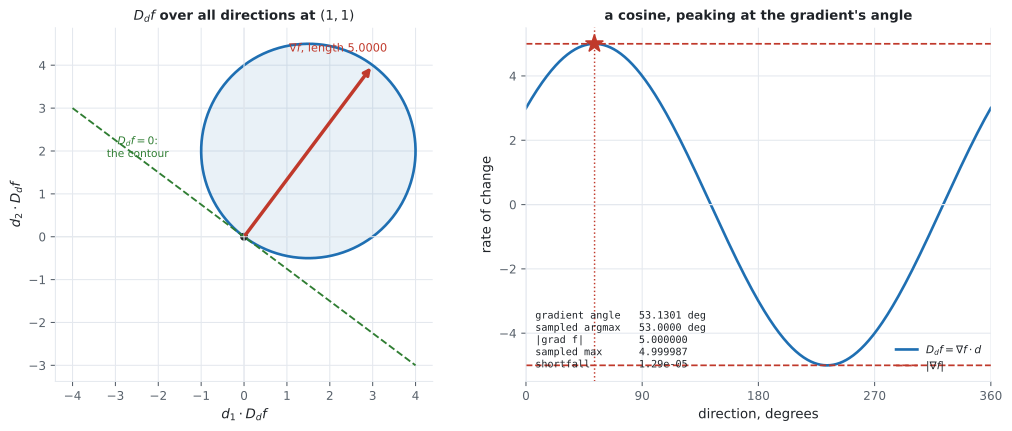
From the sweep. The left panel’s shape is the whole argument. The directional derivative is linear in , so plotted at radius rate it traces a circle through the origin. A circle through the origin has exactly one widest point, and that point is where aligns with .
Two numbers close it:
| value | |
|---|---|
| gradient angle | |
| sampled argmax over a grid | |
| sampled maximum | |
| shortfall |
Exercise 2 repeats the sweep on a -point grid: the shortfall falls to
, still not zero. Only evaluating at the exact gradient
direction gives a gap of 0.0e+00.
The shortfall is geometry, not error: a grid can only get within half a step of the true angle, and . This is the same lesson as Chapter 4’s Exercise 4.12 — sampling demonstrates the bound and never the attainment. Evaluating at the exact gradient direction gives on the nose.
The right panel adds one thing the rosette hides: the curve spends half its length below zero. Half of all directions go downhill. That is obvious once stated and it is the reason gradient descent steps along rather than searching.
From the shapes figure. The transpose count is the argument. A three-layer network is a composition of six functions; with rows that is six matrix products in the order you wrote the layers, and with columns it is six products in reverse order with a transpose on each. Both compute the same numbers. Only one of them is easy to get right at 3 a.m.
Pitfalls
Section titled “Pitfalls”Compare
Section titled “Compare”| object | shape | what it answers |
|---|---|---|
| partial derivative | scalar | how fast changes if only moves |
| gradient | the direction of fastest increase, and its rate | |
| directional derivative | scalar | how fast changes along one chosen |
| Jacobian (§5.3) | the same, for a function with outputs | |
| Hessian (§5.7) | how the gradient itself changes — curvature | |
| level set / contour | an -dimensional surface | where does not change at all |
The gradient and the contour are the same information twice: one is the direction of maximum change, the other the directions of none, and they are orthogonal complements of each other in the sense of §3.6.
-
The book gives two reasons for making the gradient a row vector. What is the practical one?
The book states this at Equation 5.53: writing the chain rule as a matrix multiplication only makes sense if the gradient is a row. Note that PyTorch does the opposite, storing gradients shaped like the parameter — so check which convention is in force before transposing.
pch.quizShowAnswer
B — The multivariate chain rule becomes a plain matrix product whose shapes chain left to right in the order the functions apply — with the column convention the same composition needs a transpose per layer and the factors come in reverse order — The book states this at Equation 5.53: writing the chain rule as a matrix multiplication only makes sense if the gradient is a row. Note that PyTorch does the opposite, storing gradients shaped like the parameter — so check which convention is in force before transposing.
-
Why do 'steepest ascent', 'the rate is the norm' and 'perpendicular to the contour' all follow from one identity?
One inner product, three corollaries. It also explains the shape of the sweep: linear in d means the polar plot is a circle through the origin, and a circle through the origin has exactly one widest point.
pch.quizShowAnswer
B — Because the directional derivative is grad f dotted with d, which equals the norm of grad f times cos theta — so the maximum is at theta = 0, its value is the norm, and it is zero at theta = 90 degrees — One inner product, three corollaries. It also explains the shape of the sweep: linear in d means the polar plot is a circle through the origin, and a circle through the origin has exactly one widest point.
-
The sampled maximum of the directional derivative came out as 4.999987 against a true 5.000000. Is that an error?
The same lesson as Exercise 4.12 in Chapter 4: sampling can demonstrate an upper bound convincingly and cannot demonstrate that the bound is attained. For attainment you evaluate at the claimed maximiser.
pch.quizShowAnswer
B — No. The sweep is on a half-degree grid, so it can only get within half a step of the true angle, and 5 times (1 minus cos 0.13 degrees) is about 1.3e-05 — exactly the observed shortfall. Evaluating at the exact gradient direction gives 5.000000 — The same lesson as Exercise 4.12 in Chapter 4: sampling can demonstrate an upper bound convincingly and cannot demonstrate that the bound is attained. For attainment you evaluate at the claimed maximiser.
-
In Example 5.7, why does optimising x1 and then x2 not reach the same place as following the gradient?
Coordinate descent is a legitimate algorithm with its own guarantees, but it is a different one. On a function with strong cross terms the gap in step count can be arbitrarily large.
pch.quizShowAnswer
B — Because the partial derivative with respect to x1 is 2 x1 x2 + x2 cubed, which depends on x2 — so changing x2 changes the best x1. The partials are not independent slopes, which is why they have to be assembled into a vector — Coordinate descent is a legitimate algorithm with its own guarantees, but it is a different one. On a function with strong cross terms the gap in step count can be arbitrarily large.
-
In the from-scratch table, the point [0.0, 0.0] gives a relative error of exactly 0.0e+00. Why, and what does it tell you about that point?
A gradient check that only ever tested critical points would pass trivially. Distinguishing a saddle from a minimum needs the Hessian, which is §5.7 — and that is exactly why §5.7 exists.
pch.quizShowAnswer
B — Both partials are exactly zero there, so both routes return zero and the difference is exactly zero. It is a critical point of Example 5.7 — and a saddle, not an optimum, which the first derivative cannot tell you — A gradient check that only ever tested critical points would pass trivially. Distinguishing a saddle from a minimum needs the Hessian, which is §5.7 — and that is exactly why §5.7 exists.
🧪 Try It Yourself
Section titled “🧪 Try It Yourself”Exercise 1 – Example 5.7, from the definition
Section titled “Exercise 1 – Example 5.7, from the definition”Exercise 2 – Sweep every direction
Section titled “Exercise 2 – Sweep every direction”Exercise 3 – Perpendicular to the level set
Section titled “Exercise 3 – Perpendicular to the level set”Exercise 4 – Example 5.8 and the chain rule as a matrix product
Section titled “Exercise 4 – Example 5.8 and the chain rule as a matrix product”Exercise 5 – Where the numeric gradient stops being trustworthy
Section titled “Exercise 5 – Where the numeric gradient stops being trustworthy”Recall card
Section titled “Recall card”- A partial derivative is Definition 5.2 with the other variables frozen, so every rule from §5.1 applies to it unchanged.
- The gradient is the row vector of all n partials, shape 1 by n — Equation 5.40 — and the book gives two reasons for the row: it generalises to vector-valued functions without a shape change, and it makes the chain rule a plain matrix product.
- One identity gives three claims. The directional derivative is grad f dotted with d, which is the norm of grad f times cos theta; so the steepest direction is the gradient’s, the steepest rate is its norm, and the contour directions give zero.
- Measured on Example 5.7 at (1,1): grad = [3, 4], norm exactly 5, angle 53.1301 degrees; a half-degree sweep finds 4.999987 at 53.0000 degrees, short by 1.29e-05 — grid geometry, not error.
- The gradient is perpendicular to the level set, and the effect is large: the same step along the gradient moves f between 2734 and 7357 times more than along the contour.
- Half of all directions go downhill, which is why descent steps along minus the gradient instead of searching.
- Equation 5.53’s chain rule is a (1 x n)(n x m) matrix product — shapes chaining left to right in the order the functions apply, no transposes.
- A NumPy 1-D array is not a row vector. Shape (2,) broadcasts either way, so a transposed Jacobian produces a plausible number rather than an error.
- Gradient checking needs a relative tolerance and a central difference. At h = 1e-6 a correct gradient lands around 1e-11 relative; at h = 1e-15 the check is 4.7e+10 times worse than at its best.
- A vanishing gradient is not a minimum. The saddle x1 squared minus x2 squared has zero gradient at the origin; telling the cases apart needs the Hessian, which is §5.7.
Next: Gradients of Vector-Valued Functions — the same row, stacked m times into a Jacobian.
pch.coffeeTagline
pch.coffeeCtapch.feedbackHeading
pch.feedbackSubheading