Interpreting What Convnets Learn (Grad-CAM)

A convnet is more inspectable than most models because its features are pictures. You can print them. That does not make the pictures trustworthy — a heat map is itself the output of a computation, and a computation can produce a convincing picture from an untrained network.

Everything here runs against one model: three convolutional blocks trained on 8,000 Fashion-MNIST rows for 15 epochs, 56,394 parameters, validation accuracy 0.7920. A deliberately mediocre model, because interpretation is a debugging tool and debugging needs mistakes to look at.

What you’ll learn

• What layer activations actually look like, and the measured way they change with depth: zero fraction 0.2071 → 0.4271, maximum 1.61 → 20.44 from the first block to the third.
• Why 4 of 64 third-block channels were silent on the image, and what that means.
• How gradient ascent synthesises a filter’s preferred input, and why one filter refused to respond at all (0.000 after 120 steps).
• Grad-CAM in nine lines of NumPy plus one GradientTape.
• Occlusion sensitivity as the slow, assumption-free check: 441 forward passes, agreeing with Grad-CAM at only 0.5697.
• The sanity check most saliency methods fail — and how far this one gets: raw peaks 375× apart, normalised maps still correlating at 0.6729.

Activations: what each layer actually responds to

The first technique needs no gradients. Build a model that outputs an intermediate layer and call predict.

A probe on any intermediate layer

probe = keras.Model(model.inputs, model.get_layer("conv1").output)
maps = probe.predict(image[None, ...], verbose=0)[0]   # (28, 28, 32)

Measured on one boot image:

Layer	Shape	Mean	Max	Zero fraction	Silent channels
conv1	(28, 28, 32)	0.0994	1.6097	0.2071	0 of 32
conv2	(14, 14, 64)	0.3567	4.2229	0.4271	0 of 64
conv3	(7, 7, 64)	2.8666	20.4410	0.3559	4 of 64

figure The six most active channels of the first and last convolutional block matplotlib

Two honest observations. First, the six busiest conv1 channels look almost identical — ranked by mean activation, early filters are largely redundant on a single image, not the tidy set of oriented edge detectors that diagrams promise. Second, by conv3 the maps are 7x7 and have stopped being pictures: they are position-coded evidence, which is exactly why Grad-CAM's output is 7x7 and blocky.

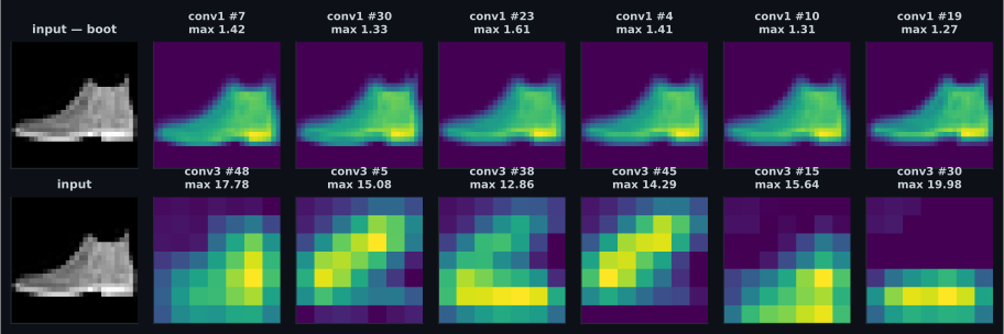
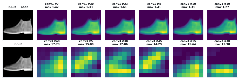
Three things in that table are worth reading carefully:

• Activations grow with depth. The maximum rises 1.61 → 4.22 → 20.44. Nothing normalises them here, and each layer adds its own scale. This is the same accumulation that broke the residual block on the architectures page.
• ReLU makes activations sparse. The zero fraction climbs from 0.2071 to 0.4271: by the second block, nearly half of all positions carry no signal at all.
• Silent channels are wasted capacity. Four conv3 channels produced nothing anywhere in the image — the filter never fires for this input. A channel silent across the entire dataset is a dead unit; a channel silent on one image is specialisation.

What a single filter is looking for

Activations tell you what a filter did on this image. Gradient ascent tells you what it wants: start from noise and change the input to maximise one channel’s mean response.

Gradient ascent on the input, not the weights

image = tf.Variable(tf.random.uniform((1, 28, 28, 1), 0.4, 0.6))
for _ in range(120):
    with tf.GradientTape() as tape:
        activation = tf.reduce_mean(probe(image, training=False)[..., channel])
    gradient = tape.gradient(activation, image)
    gradient = gradient / (tf.norm(gradient) + 1e-8)   # normalise, or it explodes
    image.assign_add(2.0 * gradient)
    image.assign(tf.clip_by_value(image, 0.0, 1.0))    # stay a valid image

The gradient is taken with respect to image; the weights never move. Two details matter and both were learned the hard way: normalising the gradient makes one step size work for every layer, and clipping keeps the result inside $[0, 1]$ so it is still an image.

Filter	Response after 120 steps	Image std	Fraction pinned at 0 or 1
conv1 #0	0.167	0.4931	0.9656
conv1 #1	0.021	0.1934	0.1378
conv1 #2	0.147	0.4959	0.9821
conv3 #0	0.000	0.0576	0.0000
conv3 #1	17.526	0.4783	0.9375
conv3 #2	12.838	0.4782	0.8520

figure Inputs synthesised to maximise one filter each matplotlib

The four that worked are stripe patterns at different orientations and scales, and the deeper ones are visibly coarser — a bigger receptive field means a bigger stripe. The two flat panels are the interesting ones: conv3 filter 0 never rose above 0.000 in 120 steps, and its image stayed at std 0.0576. There is nothing to ascend when the gradient is zero everywhere, which is what a permanently dead ReLU channel looks like from the outside.

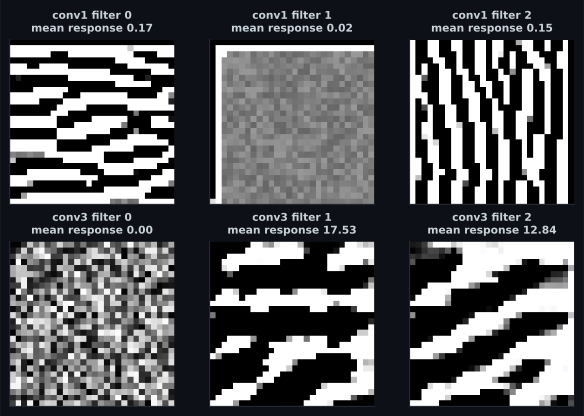
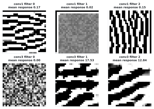
The pinned fraction (0.9656, 0.9821, 0.9375) says the successful ascents ran straight into the clipping bounds — the filter wants more contrast than an image can carry. That is normal, and it is why published filter visualisations add a smoothness penalty or blur between steps: without one, you get maximum-contrast stripes rather than anything a photograph would contain.

Grad-CAM

Activations and filter maximisation are class-agnostic. Grad-CAM answers the question you actually have when a prediction is wrong: which positions drove this class?

The recipe, in full:

$$\alpha_k = \frac{1}{HW}\sum_{i,j} \frac{\partial y_c}{\partial A^k_{ij}} \qquad L = \mathrm{ReLU}\!\left(\sum_k \alpha_k A^k\right)$$

$A^k$ is the $k$-th channel of the last convolutional layer, $y_c$ is the score for class $c$. The weight $\alpha_k$ is the average gradient of that score with respect to the channel — how much this channel matters, globally. The map is the weighted sum of channels, with negative evidence discarded by the ReLU.

Grad-CAM

probe = keras.Model(model.inputs, [model.get_layer("conv3").output, model.output])
with tf.GradientTape() as tape:
    maps, predictions = probe(image[None, ...], training=False)
    score = predictions[:, class_index]
gradient = tape.gradient(score, maps)[0].numpy()
weights = gradient.mean(axis=(0, 1))                       # one alpha per channel
heat = np.maximum((maps[0].numpy() * weights).sum(axis=-1), 0)
heat = heat / (heat.max() + 1e-8)

The output is 7×7 — the spatial size of conv3, upsampled for display. Grad-CAM cannot be sharper than the layer it reads, which is the price of reading a layer deep enough to know what a class is.

figure Grad-CAM for three correct and three incorrect predictions matplotlib

The correct row is unsurprising — the trousers prediction (confidence 0.9998) sits on a vertical band exactly where the legs are. The wrong row is where the technique earns its keep: the coat called 'trouser' (0.3479) is being read down its central vertical opening, which really does look like the gap between two legs at 7x7 resolution, and the bag called 'boot' (0.5904) is being read at its strap. The model is not hallucinating; it is looking at a real feature and drawing the wrong conclusion from it.

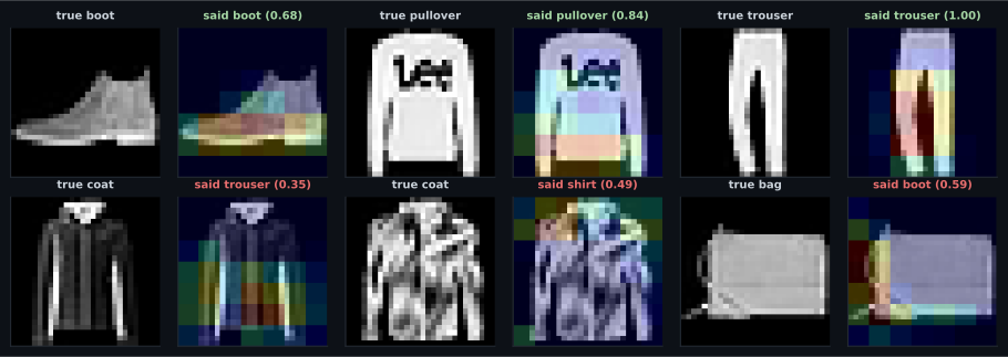
Prediction	True	Said	Confidence	Heat map centre mass
correct	boot	boot	0.6820	0.3448
correct	pullover	pullover	0.8352	0.3260
correct	trouser	trouser	0.9998	0.4151
wrong	coat	trouser	0.3479	0.3391
wrong	coat	shirt	0.4911	0.1229
wrong	bag	boot	0.5904	0.2067

The sanity check

Here is the part that most tutorials skip. Grad-CAM produces a plausible-looking heat map from a network with random weights, because a weighted sum of random feature maps is still a smooth blob with a peak somewhere. If you never compare against that baseline, you cannot distinguish “the model looks here” from “this arithmetic produces blobs”.

The check to run before you trust any saliency map

trained_map = gradcam(model, image, class_index)
random_map = gradcam(freshly_initialised_model, image, class_index)
print(np.corrcoef(trained_map.ravel(), random_map.ravel())[0, 1])

Exercise 5 runs it, and the answer is uncomfortable in a useful way:

	Raw peak before normalising	Cells above 0.1
trained	0.0761	17 of 49
untrained	0.0002	31 of 49

The raw magnitudes differ by 375× — training clearly changed something. But the normalised maps still correlate at 0.6729, which means roughly two thirds of the shape of a Grad-CAM picture here comes from the architecture and the arithmetic rather than from what the network learned.

Both halves matter. Normalisation is what makes the map displayable, and it is also what throws away the evidence that the trained map is 375× stronger. If you publish a normalised heat map without this comparison, you are showing a picture that an untrained network largely reproduces.

The complementary check is occlusion sensitivity: slide a grey patch over the image and record how far the confidence falls. It makes no assumption about gradients, layers or linearity — it just deletes information and measures the consequence. It costs one forward pass per position (441 for an 8×8 patch on 28×28, Exercise 3), which is exactly why Grad-CAM exists.

diagram Diagram mermaid

  flowchart TB
  A["a prediction you don't trust"] --> B{"is it wrong,
or just unexplained?"}
  B -->|"wrong"| C["Grad-CAM on the predicted class
and on the true class"]
  B -->|"unexplained"| D["Grad-CAM on the predicted class"]
  C --> E["do the two maps
look at the same place?"]
  E -->|"yes"| F["the feature is ambiguous
— more data or resolution"]
  E -->|"no"| G["the model is reading
the wrong region"]
  D --> H["occlusion sensitivity
to confirm"]
  G --> H
  H --> I["sanity check against
random weights"]

sketch Grad-CAM as a weighted sum p5.js Pause Restart

Drag the four alpha weights and watch the heat map change. This is the entire method — one weight per channel, then ReLU.

sketch The measured table, ranked p5.js Pause Restart

Click a column to rank every row by it. The bars are that column's values and the highest and lowest are computed from the numbers, not written in.

Pitfalls

• Trusting a heat map without the random-weights check. Measured here, the trained and untrained normalised maps correlate at 0.6729 — most of the picture’s shape is architectural.
• Normalising away the evidence. The trained map’s raw peak was 375× the untrained one’s (0.0761 against 0.0002); dividing by the maximum discards exactly that.
• Reading Grad-CAM as pixel-level evidence. The map here is 7×7 upsampled to 28×28; every “region” is a 4×4 block.
• Taking Grad-CAM from the wrong layer. Too early and it has no class information; too late (after global pooling) and it has no positions.
• Explaining only the predicted class. For a wrong prediction, also compute the map for the true class — the comparison is the diagnosis.
• Concluding a filter is broken from one gradient-ascent failure. conv3 filter 0 returned 0.000, which is consistent with a dead channel; confirm it across images before believing it.
• Publishing raw gradient-ascent images as “what the filter sees”. 0.9656 of the pixels were pinned at the clipping bounds. Without a smoothness penalty these are adversarial-contrast patterns, not natural features.
• Interpreting a model you have not validated. This one scores 0.7920. An explanation of a bad model explains bad behaviour.

Recap

• An intermediate probe is keras.Model(model.inputs, layer.output) — no gradients needed.
• Activations grew from max 1.61 (conv1) to 20.44 (conv3) with the ReLU zero fraction rising 0.2071 → 0.4271, and 4 of 64 conv3 channels were silent on the test image.
• Gradient ascent on the input synthesises a filter’s preferred stimulus; two of six filters failed, one of them (0.000 response) consistent with a dead channel.
• Grad-CAM = average gradient per channel → weighted sum of channels → ReLU. Nine lines, resolution fixed by the layer you read.
• Wrong predictions were readable: a coat called “trouser” was being read down its central opening; a bag called “boot” at its strap.
• The random-weights check gave raw peaks of 0.0761 against 0.0002 but normalised maps correlating at 0.6729 — run it, and report both numbers.
• Occlusion sensitivity cost 441 forward passes for one 28×28 image, agreed with Grad-CAM at 0.5697, and found a region whose removal raised confidence by 0.0534 — something a gradient map cannot express.

Next

Segmentation labelled every pixel and Grad-CAM located a class approximately. Boxes are the middle ground, and they need a different output format entirely: Object Detection (Bounding Boxes and YOLO).

pch.quizTag pch.quizDefaultTitle

1. Grad-CAM on this model produces a 7x7 map for a 28x28 input. Why not 28x28?

   A Because the heat map is always downsampled by 4 for display B Because it reads the last convolutional layer, whose spatial size is 7x7 after two pooling steps — resolution is bounded by the layer you take gradients at C Because the ReLU discards three quarters of the positions D Because gradients are only defined at pooled positions
   pch.quizShowAnswer

   B — Because it reads the last convolutional layer, whose spatial size is 7x7 after two pooling steps — resolution is bounded by the layer you take gradients at — Taking the map from an earlier layer gives more resolution and less class information. That trade-off is the method's main limitation.

2. Gradient ascent on conv3 filter 0 returned a mean response of 0.000 after 120 steps, and the synthesised image stayed at std 0.0576. What is the most likely explanation?

   A The learning rate of 2.0 was too small B The channel is dead — a ReLU that outputs zero for every input has zero gradient, so there is nothing for ascent to climb C 120 steps is not enough for a deep layer D The image needed to be initialised from a real photograph
   pch.quizShowAnswer

   B — The channel is dead — a ReLU that outputs zero for every input has zero gradient, so there is nothing for ascent to climb — The measurement backs it up: 4 of 64 conv3 channels produced no activation anywhere on the test image either.

3. What does the random-weights sanity check tell you?

   A Whether the model has converged B Whether the saliency map depends on what the model learned, rather than on the architecture and the arithmetic of the method C Whether the input image is in distribution D Whether the learning rate was correct
   pch.quizShowAnswer

   B — Whether the saliency map depends on what the model learned, rather than on the architecture and the arithmetic of the method — A weighted sum of random feature maps is still a smooth blob with a peak. If the trained and random maps agree, the map is not evidence about the model.

4. The zero fraction of activations rose from 0.2071 in conv1 to 0.4271 in conv2. What causes it?

   A Max pooling discarding values B The ReLU: every negative pre-activation becomes exactly zero, and deeper layers have more negative pre-activations C Numerical underflow in float32 D Dropout, which is active during prediction
   pch.quizShowAnswer

   B — The ReLU: every negative pre-activation becomes exactly zero, and deeper layers have more negative pre-activations — Sparsity is a feature of ReLU networks, not a bug — but a channel that is zero for every input is a dead unit and pure waste.

5. Occlusion sensitivity needed 441 forward passes for one 28x28 image with an 8x8 patch. When is that worth paying?

   A Never — Grad-CAM is strictly better B When you need an explanation that makes no assumption about gradients or layer choice, for example to check a Grad-CAM map you are about to act on C Only for models without convolutional layers D Only when the model is untrained
   pch.quizShowAnswer

   B — When you need an explanation that makes no assumption about gradients or layer choice, for example to check a Grad-CAM map you are about to act on — It measures the thing you actually care about — what happens to the prediction when information is removed — at a cost that scales with image area.

🧪 Try It Yourself

pch.exerciseTag pch.exerciseTitle

pch.exerciseTag pch.exerciseTitle

pch.exerciseTag pch.exerciseTitle

pch.exerciseTag pch.exerciseTitle

pch.exerciseTag pch.exerciseTitle