
Recommender Systems from Scratch
What you’ll learn
Section titled “What you’ll learn”- why the empty cells of a user-item matrix are the target, not missing data
- the popularity baseline, which is not a straw man: hit rate 0.1976 at 10
- item-item collaborative filtering in six lines of numpy: 0.3481
- BPR matrix factorisation by SGD, and why it lost here: 0.3196
- the evaluation trap that doubles every published number: 100 sampled negatives
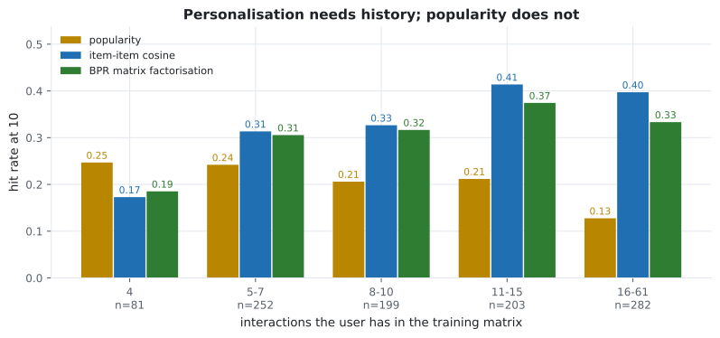
- cold start, measured: with 4 interactions, popularity beats personalisation 0.25 to 0.17
Implicit feedback
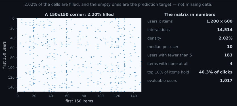
Section titled “Implicit feedback”The data is 1,200 users, 600 items, and a 1 wherever a user interacted with an item. Generated from latent factors plus an item popularity term, so the reason any cell is filled is known — which lets us separate “the model learned taste” from “the model learned what is popular”.
| Quantity | Value |
|---|---|
| users × items | 1,200 × 600 |
| interactions | 14,514 |
| density | 2.02% |
| median interactions per user | 10 |
| users with fewer than 5 | 183 |
| items with none at all | 4 |
| top 10% of items hold | 40.3% of all interactions |
The long tail, and why popularity is hard to beat
Section titled “The long tail, and why popularity is hard to beat”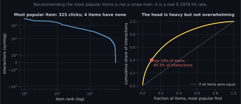
Evaluation, before any model
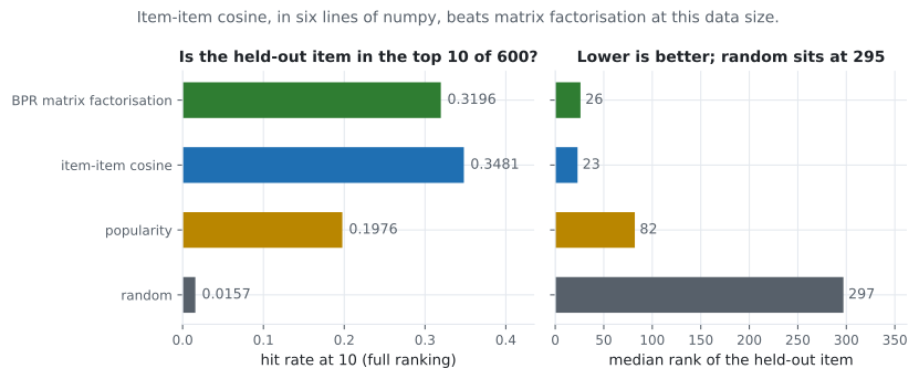
Section titled “Evaluation, before any model”Leave-one-out: for every user with at least 5 interactions, hide one at random. That gives 1,017 evaluable users. Then, for each of them, rank all 600 items — excluding the ones they already interacted with in training — and ask where the hidden item landed.
With one held-out item per user, NDCG reduces to a rank-discounted hit rate: it rewards position 1 over position 9, which hit rate does not.
Four scorers
Section titled “Four scorers”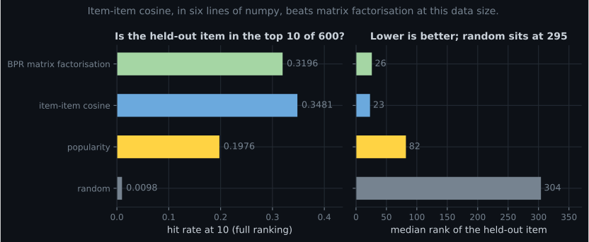
| Scorer | Hit@10 | NDCG@10 | Median rank |
|---|---|---|---|
| random | 0.0098 | 0.0051 | 304 |
| popularity | 0.1976 | 0.0975 | 82 |
| item-item cosine | 0.3481 | 0.2024 | 23 |
| BPR matrix factorisation | 0.3196 | 0.1776 | 26 |
Item-item collaborative filtering
Section titled “Item-item collaborative filtering”The whole method, once the matrix is in memory:
norms = np.linalg.norm(train, axis=0)          # column norms = item popularity
norms[norms == 0] = 1.0                        # unseen items: avoid dividing by 0
unit = train / norms                           # L2-normalise each item column
similarity = unit.T @ unit                     # cosine between every item pair
np.fill_diagonal(similarity, 0.0)              # an item is not its own neighbour

scores = train[user] @ similarity               # sum of similarities to what you took
The last line is the recommendation: an item scores highly if it is similar to the items this user already interacted with. No optimisation, no hyperparameters, no training loop. On this data it is the best of the four.
Two properties are worth knowing. The cosine normalisation is what stops popular items dominating —
without it, train[user] @ train.T @ train is essentially a popularity ranking. And the similarity
matrix is here but in general, so at a million items you need approximate
neighbours (NearestNeighbors with a tree, FAISS, ScaNN) instead of a dense product.
BPR matrix factorisation
Section titled “BPR matrix factorisation”Matrix factorisation learns a vector per user and per item such that the dot product ranks correctly. The BPR objective takes a seen item and an unseen item and pushes them apart:
def bpr(train, k=16, epochs=30, lr=0.05, reg=0.01, seed=1):
    """Rank a seen item above a randomly drawn unseen one, by SGD."""
    rng = np.random.default_rng(seed)
    n_users, n_items = train.shape
    P = rng.normal(0, 0.1, (n_users, k))
    Q = rng.normal(0, 0.1, (n_items, k))
    pairs = np.argwhere(train == 1)

    for _ in range(epochs):
        rng.shuffle(pairs)
        for u, i in pairs:
            j = int(rng.integers(0, n_items))          # sample a negative
            while train[u, j] == 1:
                j = int(rng.integers(0, n_items))
            gradient = 1.0 / (1.0 + np.exp(P[u] @ (Q[i] - Q[j])))
            pu, qi, qj = P[u].copy(), Q[i].copy(), Q[j].copy()
            P[u] += lr * (gradient * (qi - qj) - reg * pu)
            Q[i] += lr * (gradient * pu - reg * qi)
            Q[j] += lr * (-gradient * pu - reg * qj)
    return P, Q
It reached 0.3196 after 30 epochs over 13,497 positive pairs — and 0.2281 after 10 epochs, which is worth knowing before you conclude that factorisation does not work. It is an iterative method and it needs its iterations.
Why it still loses to a six-line neighbourhood method here: 13,497 interactions is not much data for 1,800 factor vectors. At 16 factors, BPR is fitting 1,200 × 16 + 600 × 16 = 28,800 parameters from 13,497 observations. Item-item cosine fits nothing. The ordering reverses on real catalogues with millions of interactions, where factorisation generalises across the sparsity in a way neighbourhoods cannot — but “matrix factorisation is better” is a statement about data volume, not about algorithms.
The evaluation trap
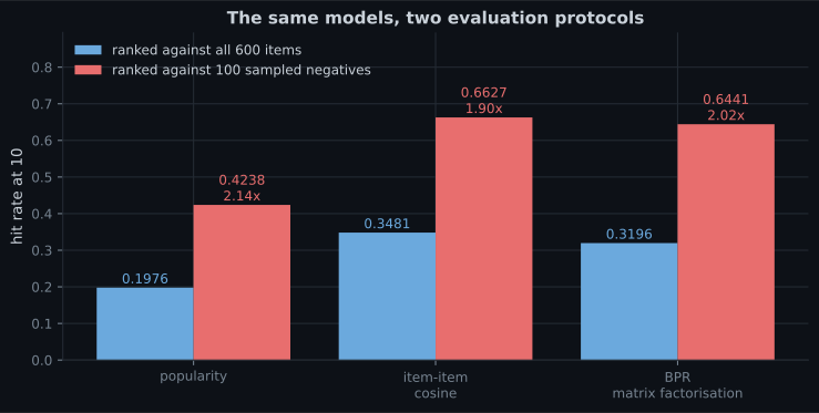
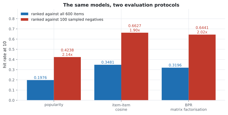
Section titled “The evaluation trap”Ranking the held-out item against all items is expensive, so a very common shortcut is to rank it against a sample of 100 unseen items. Here is what that does:
| Scorer | Full ranking (600 items) | 100 sampled negatives | Inflation |
|---|---|---|---|
| popularity | 0.1976 | 0.4238 | 2.14× |
| item-item cosine | 0.3481 | 0.6627 | 1.90× |
| BPR matrix factorisation | 0.3196 | 0.6441 | 2.01× |
The arithmetic is straightforward — being in the top 10 of 101 candidates is far easier than the top 10 of 600 — but two consequences are not:
- Cross-paper comparison breaks. A published 0.66 and your 0.35 may be the same model.
- The ranking can change. The inflation is not a constant factor: it depends on how a model distributes scores over the tail. Krichene and Rendle showed in 2020 that sampled metrics can reorder methods, which is why full ranking (or a documented, fixed candidate set) is now expected.
If you must sample for speed, sample the same negatives for every model and say so in the report.
Cold start, measured
Section titled “Cold start, measured”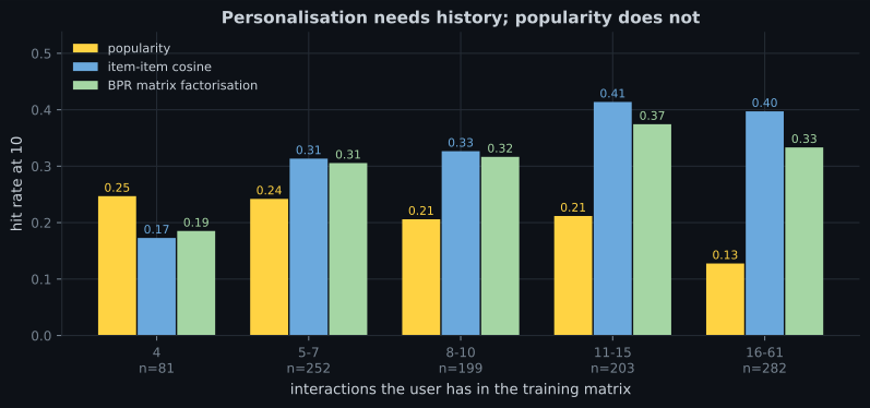
| Interactions in training | n | popularity | item-item | BPR |
|---|---|---|---|---|
| 4 | 81 | 0.25 | 0.17 | 0.19 |
| 5–7 | 252 | 0.24 | 0.31 | 0.31 |
| 8–10 | 199 | 0.21 | 0.33 | 0.32 |
| 11–15 | 203 | 0.21 | 0.41 | 0.37 |
| 16–61 | 282 | 0.13 | 0.40 | 0.33 |
Both halves of this table are load-bearing.
Personalisation loses on cold users. With four interactions there is not enough signal, and the best available guess is what everyone else likes. This is why production systems are almost always a blend: popularity (or editorial curation) for new users, collaborative filtering once history accumulates, usually with a smooth interpolation rather than a switch.
Popularity gets worse as users get more active — 0.25 down to 0.13 — because the recommendation excludes items the user already has, and heavy users have consumed most of the head. An aggregate hit rate hides both effects. Always segment by activity.
Note also the 183 users with fewer than five interactions who were excluded from evaluation entirely. They are 15% of the user base, they are the hardest cases, and every leave-one-out benchmark quietly drops them. Their existence is a product problem, not a modelling one.
What to serve whom
Section titled “What to serve whom”The measured table above is a routing policy waiting to be written down:
  flowchart TD
  R["A request for recommendations"] --> A{"How many interactions
does this user have?"}
  A -->|"0 -- brand new"| Z["Editorial or popularity.
No model can help;
collect signal instead."]
  A -->|"1 to 4"| P["Popularity.
Measured 0.25 against
0.17 for item-item."]
  A -->|"5 to 15"| M["Personalised: item-item
cosine, 0.31 to 0.41"]
  A -->|"16 or more"| M2["Personalised, and drop
popularity entirely --
it decays to 0.13"]
  P --> B{"Blend or switch?"}
  M --> B
  M2 --> B
  B -->|"switch at a hard
threshold"| B1["Visible jump in the feed
the day a user crosses it"]
  B -->|"interpolate on
interaction count"| B2["Preferred: score =
w(n) * personal + (1-w(n)) * popular"]
  B1 --> E["Evaluate per bucket,
never in aggregate"]
  B2 --> E
  E --> F{"Reporting a number
to anyone?"}
  F -->|"yes"| G["State the protocol:
full ranking over all items,
or a fixed sampled candidate set.
Sampling roughly doubled every
hit rate here."]
Two of those boxes exist only because of measurements on this page: the 1-to-4 bucket routes to popularity because personalisation loses there, and the reporting box exists because the same three models scored between 1.90× and 2.14× higher under sampled evaluation. Neither is a design preference; both are what the numbers said.
See it move
Section titled “See it move”Item-item cosine is one formula, and the effect of normalisation is easiest to feel by toggling it. Below, five users have interacted with six items; the similarity between two items is the cosine of their columns.
Fill an entire column — make one item universally popular — and watch what happens. Under raw co-occurrence that item becomes the most similar item to everything, so it is recommended to everybody. Under cosine it does not, because the normalisation divides by its own norm. That single division is the difference between a recommender and a bestseller list.
Pitfalls
Section titled “Pitfalls”| Pitfall | Why it bites | What to do |
|---|---|---|
| Treating zeros as negatives | 97.98% of cells are zero; the model learns to say no | BPR, negative sampling or weighted ALS |
| Skipping the popularity baseline | It scores 0.1976 at 10 here, unpersonalised | Always report it alongside your model |
| Sampled negatives in the metric | Inflated 1.90× to 2.14×, non-uniformly | Rank against everything, or fix and document the candidate set |
| Recommending items the user already has | Trivially “correct” and useless | Mask known items before ranking |
| One aggregate hit rate | Popularity wins at 4 interactions and loses at 16 | Segment by user activity |
| Ignoring the excluded users | 183 users (15%) had too little history to evaluate | Report the coverage, and design for them explicitly |
| Un-normalised similarity | Popular items become everyone’s nearest neighbour | Cosine, or shrinkage on the counts |
| Concluding MF beats neighbourhoods (or vice versa) | 0.3196 against 0.3481 here at 13.5k interactions | Measure both at your data volume |
- The matrix is 1,200 × 600 and 2.02% filled; the zeros are the prediction target, not missing data.
- The top 10% of items hold 40.3% of interactions, which is why popularity reaches 0.1976 at 10 with no personalisation.
- Item-item cosine, six lines of numpy, reached 0.3481 and median rank 23 of 600.
- BPR matrix factorisation reached 0.3196 after 30 epochs and 0.2281 after 10 — it lost here because 13,497 interactions is thin for 28,800 parameters.
- Ranking against 100 sampled negatives inflated hit rate by 1.90× to 2.14×, non-uniformly.
- With four interactions, popularity beat personalisation 0.25 to 0.17; with 16 or more it lost 0.13 to 0.40.
-
Your user-item matrix is 97.98% zeros. How should the zeros be treated?
Training on all 691,486 zeros as negatives teaches the model to predict 'no', which is right 97.98% of the time and worthless. BPR sidesteps it by only ever comparing a seen item against an unseen one.
pch.quizShowAnswer
B — As unlabelled: a zero mixes dislike, ignorance and not-yet, so use an implicit-feedback objective, negative sampling or weighted ALS — Training on all 691,486 zeros as negatives teaches the model to predict 'no', which is right 97.98% of the time and worthless. BPR sidesteps it by only ever comparing a seen item against an unseen one.
-
Your new model reaches hit rate at 10 of 0.30. Is it good?
Two references are missing: the unpersonalised baseline and the candidate set. Both change the interpretation by a factor of two here, and neither is visible in the number itself.
pch.quizShowAnswer
B — Unknown until you compare against popularity (0.1976 here) and state the evaluation protocol — the same model scores 0.64 against 100 sampled negatives — Two references are missing: the unpersonalised baseline and the candidate set. Both change the interpretation by a factor of two here, and neither is visible in the number itself.
-
Item-item cosine (0.3481) beat BPR matrix factorisation (0.3196) on this data. What does that establish?
BPR also improved from 0.2281 at 10 epochs to 0.3196 at 30, so it was still learning. The transferable lesson is procedural: implement the cheap neighbourhood baseline first, because it may win at your scale.
pch.quizShowAnswer
B — At 13,497 interactions, fitting 28,800 factor parameters is data-starved — the ordering is about data volume, and would likely reverse on a large catalogue — BPR also improved from 0.2281 at 10 epochs to 0.3196 at 30, so it was still learning. The transferable lesson is procedural: implement the cheap neighbourhood baseline first, because it may win at your scale.
-
Why does the popularity baseline get WORSE for more active users, from 0.25 down to 0.13?
Masking known items is correct — recommending something already purchased is worthless — and it systematically strips popularity of its best candidates for heavy users. It is also why an aggregate hit rate hides the cold-start problem entirely.
pch.quizShowAnswer
B — Known items are excluded from the ranking, and active users have already consumed most of the popular head — Masking known items is correct — recommending something already purchased is worthless — and it systematically strips popularity of its best candidates for heavy users. It is also why an aggregate hit rate hides the cold-start problem entirely.
-
A paper reports hit rate at 10 of 0.66 using 100 sampled negatives. Your full-ranking evaluation gives 0.35. What can you conclude?
The inflation is real, large and model-dependent, which means it can reorder methods rather than shifting them all equally. Reproduce their protocol or rank against the full catalogue; do not compare across protocols.
pch.quizShowAnswer
B — Nothing about relative quality — the protocols differ, and here the same models moved by 1.90x to 2.14x under exactly that change — The inflation is real, large and model-dependent, which means it can reorder methods rather than shifting them all equally. Reproduce their protocol or rank against the full catalogue; do not compare across protocols.
🧪 Try It Yourself
Section titled “🧪 Try It Yourself”Exercise 1 – Build the interaction matrix
Section titled “Exercise 1 – Build the interaction matrix”Exercise 2 – Leave one out, then try popularity
Section titled “Exercise 2 – Leave one out, then try popularity”Exercise 3 – Item-item cosine in six lines
Section titled “Exercise 3 – Item-item cosine in six lines”Exercise 4 – BPR by hand
Section titled “Exercise 4 – BPR by hand”Exercise 5 – Reproduce the sampled-negatives inflation
Section titled “Exercise 5 – Reproduce the sampled-negatives inflation”Anomaly and Outlier Detection — the last applied problem, and the only one where you usually have no labels at all, which changes what “evaluation” can even mean.
pch.coffeeTagline
pch.coffeeCtapch.feedbackHeading
pch.feedbackSubheading