What you’ll learn

• point-in-time correctness, measured: 0.7060 honest against 0.9564 when the window ends late
• six ways a serving path computes “the same” feature differently, and what each one costs
• why accuracy can fall 0.0891 while AUC falls only 0.0207 — and which one production feels
• the parity test that catches skew before a model is involved at all
• what a feature store actually buys you, and what it does not
• the one-function rule, and where it has to be enforced

The setup

An event log — 4,000 customers, 51,965 events over the 120 days before a cutoff, and 9,351 events in the 30 days after it. The label is churn in that following month, and 41.60% of customers churn. Three features, all aggregates over a 30-day window ending at the cutoff:

def window_features(events, window_days, asof, customer_ids):
    """Aggregate the log over (asof - window, asof]. One function, both paths."""
    lower = asof - pd.Timedelta(days=window_days)
    window = events[(events["ts"] > lower) & (events["ts"] <= asof)]
    grouped = window.groupby("customer").agg(events=("amount", "size"),
                                             mean_amount=("amount", "mean"),
                                             last=("ts", "max"))
    grouped["days_since"] = (asof - grouped["last"]).dt.days
 
    frame = grouped.drop(columns="last").reindex(customer_ids)
    frame["events"] = frame["events"].fillna(0)          # no events in the window
    frame["mean_amount"] = frame["mean_amount"].fillna(0)
    frame["days_since"] = frame["days_since"].fillna(999)  # the "never" sentinel
    return frame

def window_features(events, window_days, asof, customer_ids):
    """Aggregate the log over (asof - window, asof]. One function, both paths."""
    lower = asof - pd.Timedelta(days=window_days)
    window = events[(events["ts"] > lower) & (events["ts"] <= asof)]
    grouped = window.groupby("customer").agg(events=("amount", "size"),
                                             mean_amount=("amount", "mean"),
                                             last=("ts", "max"))
    grouped["days_since"] = (asof - grouped["last"]).dt.days
 
    frame = grouped.drop(columns="last").reindex(customer_ids)
    frame["events"] = frame["events"].fillna(0)          # no events in the window
    frame["mean_amount"] = frame["mean_amount"].fillna(0)
    frame["days_since"] = frame["days_since"].fillna(999)  # the "never" sentinel
    return frame

568 of 4,000 customers have no events in the window, which is why the fill values are part of the feature definition rather than an implementation detail. A serving path that fills days_sincedays_since with 0 instead of 999 has changed the feature, not the plumbing.

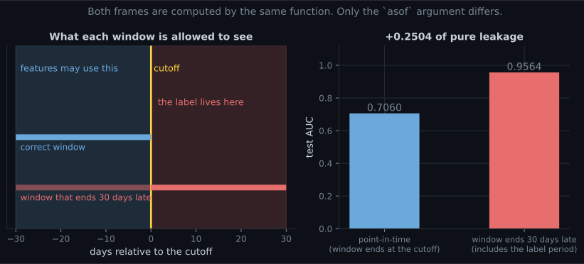
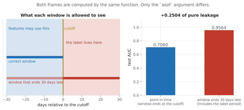
Point-in-time correctness

The asofasof argument is the whole of point-in-time correctness. Move it 30 days forward — so the window covers the month the label is about — and the model becomes spectacular:

figure+0.2504 of pure leakagematplotlib

This is the most expensive bug in applied ML, and it is almost never written as asof = cutoff + 30asof = cutoff + 30. It arrives as:

• a feature table rebuilt nightly from the current state of a customer, then joined to old labels
• df.groupby("customer")["amount"].mean()df.groupby("customer")["amount"].mean() over the whole history, with no window at all
• an aggregate maintained by the application, read at training time from the live database
• a “days since last login” column that was computed when the training set was assembled, not as of the prediction moment

Every one of these produces a number that cannot exist at prediction time. The defence is structural: compute features with a function that takes asofasof as an argument, and pass the prediction timestamp into it. A feature pipeline that cannot answer “as of when?” is not a feature pipeline.

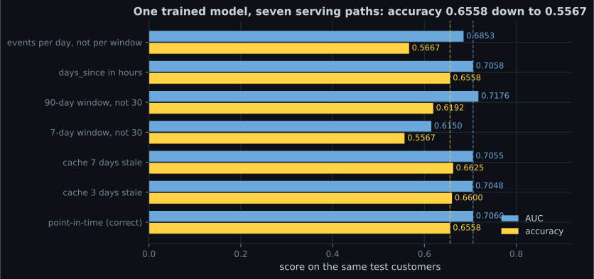
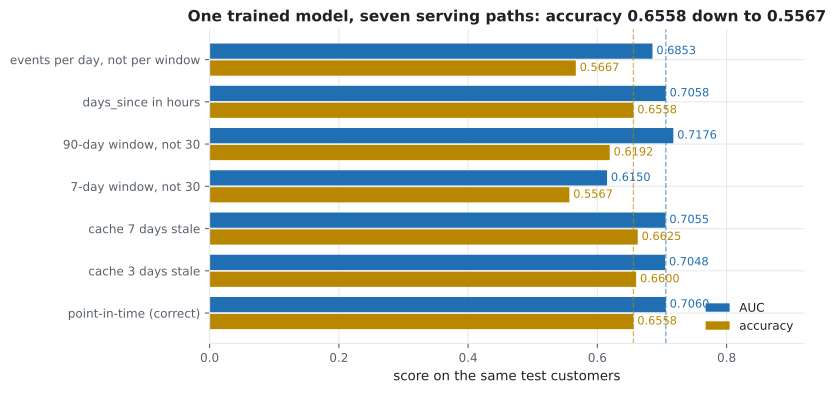
Six serving paths, one model

Now assume the training features are correct and the serving implementation differs. Same model, same test customers, six variants of the feature computation:

figureOne trained model, seven serving paths: accuracy 0.6558 down to 0.5567matplotlib

Four things worth extracting.

Staleness was harmless — here. A cache three or seven days behind changed accuracy by less than 0.007, because a 30-day count barely moves in a week. That is a property of this feature, not a general result: a “transactions in the last hour” feature served from a daily batch would be catastrophic. The test is whether the window is long relative to the staleness.

Window length is the dangerous parameter. Serving a 7-day count to a model trained on 30-day counts cost 0.0991 accuracy — a bigger loss than most modelling changes will ever gain. And nothing errors: the column is present, numeric, non-null and plausible.

A monotone rescaling can be nearly invisible in AUC and expensive in accuracy. Dividing eventsevents by 30 moved AUC by 0.0207 and accuracy by 0.0891. AUC only cares about the ranking; the threshold is calibrated to the original scale, so a rescaled input moves every prediction across it. If your monitoring watches AUC only, this class of bug is close to undetectable.

days_sincedays_since in hours cost exactly nothing. With three features and a linear model, that particular rescaling happened to preserve both ranking and the decision. Not a reason to relax: the same change on a tree ensemble, or interacting with a regularisation penalty, need not be benign. It is a reminder that the size of a skew’s damage is not predictable from the size of the code change.

See it move

The sketch is the dashboard that would have been on the wall. It cycles the seven serving paths from the table and plots each one as a point in AUC–accuracy space, keeping the correct path marked. What you are looking for is how often the two axes disagree — because a monitoring setup that watches one of them is blind to a whole class of skew.

The purple point is the whole argument for parity testing rather than metric monitoring. If your alert threshold is on AUC, the 90-day window looks like an improvement of 0.0116 while it quietly costs 0.0366 of accuracy; if your alert is on accuracy, you see a regression with no cause anywhere in the model, the data volumes, or the label distribution — because the cause is a number 3030 that became a 9090 in a different repository.

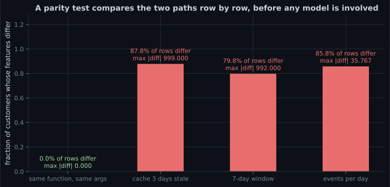
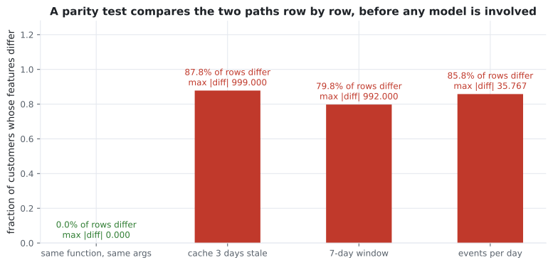
The parity test

The fix is not cleverness, it is a test. Compute the features both ways and compare them row by row, before any model is involved:

figureA parity test compares the two paths row by row, before any model is involvedmatplotlib

def test_offline_online_parity():
    """The two feature paths must agree exactly on a sample of real entities."""
    ids = sample_customer_ids(500)
    asof = pd.Timestamp("2024-04-01")
 
    offline = window_features(events_warehouse, 30, asof, ids)   # training path
    online = fetch_features_from_service(ids, asof)              # serving path
 
    assert list(offline.columns) == list(online.columns)
    mismatch = ~np.isclose(offline.to_numpy(float), online.to_numpy(float),
                           rtol=1e-9, atol=1e-9)
    offenders = offline.index[mismatch.any(axis=1)]
    assert len(offenders) == 0, (
        f"{len(offenders)} of {len(ids)} entities differ; "
        f"first: {offenders[:5].tolist()}")

def test_offline_online_parity():
    """The two feature paths must agree exactly on a sample of real entities."""
    ids = sample_customer_ids(500)
    asof = pd.Timestamp("2024-04-01")
 
    offline = window_features(events_warehouse, 30, asof, ids)   # training path
    online = fetch_features_from_service(ids, asof)              # serving path
 
    assert list(offline.columns) == list(online.columns)
    mismatch = ~np.isclose(offline.to_numpy(float), online.to_numpy(float),
                           rtol=1e-9, atol=1e-9)
    offenders = offline.index[mismatch.any(axis=1)]
    assert len(offenders) == 0, (
        f"{len(offenders)} of {len(ids)} entities differ; "
        f"first: {offenders[:5].tolist()}")

Two design notes that make this test practical:

Run it on real entity ids, not synthetic ones. The interesting disagreements are in the awkward cases — the 568 customers with no events, the ones with a single event on the boundary, the ones created yesterday.

Assert exact equality, not “close enough”. A tolerance of 1e-9 catches a changed fill value; a tolerance of 0.01 hides it. If the two paths cannot agree to floating-point noise, they are computing different features and you want to know why.

What a feature store is, minus the marketing

A feature store is three things, and only the first is conceptually interesting:

The single-definition property is the one that removes the failures on this page. A feature store gives it to you by construction, but so does a function in a shared library that both paths import — which is the right answer for most teams, and stays the right answer until you have enough features and enough consumers that discovery becomes the bottleneck.

What a feature store does not do:

• It does not stop you writing a leaky definition. asofasof correctness is still yours to get right; the store just makes the point-in-time join available.
• It does not remove the need for a parity test. Materialisation paths can still diverge — and the point-in-time join is itself code that can be wrong.
• It does not fix staleness. A TTL is a decision about how wrong you are willing to be, and it has to be set per feature: 30-day counts tolerated a week here, a one-hour count would not.

  flowchart TD
  A["A feature definition
one function, asof argument"] --> B["Offline materialisation
for training, point-in-time"]
  A --> C["Online materialisation
for serving, current values"]
  B --> D["Train"]
  C --> E["Serve"]
  D --> F["Parity test in CI:
same entities, same asof,
assert exact equality"]
  E --> F
  F -->|"fails"| G["The two paths compute
different features.
Fix before shipping."]
  F -->|"passes"| H["Log the served feature
values with the prediction"]
  H --> I["Compare distributions
weekly against training.
Skew that appears later
shows up here."]

The last box matters as much as the test: log the feature values you actually served. Given those, skew is a query rather than an investigation — you can compare served values against the training distribution, and re-score old requests with the offline path to find the divergence. Without them, a metric regression caused by skew is nearly impossible to attribute.

Pitfalls

Recap

• 4,000 customers, 51,965 events before the cutoff and 9,351 after; churn rate 0.4160; 568 customers with no events in the 30-day window.
• Moving the window 30 days later inflated AUC from 0.7060 to 0.9564 — +0.2504 of pure leakage.
• Serving a 7-day window to a 30-day model cost 0.0991 accuracy; nothing raised.
• Dividing eventsevents by 30 cost 0.0891 accuracy while AUC moved only 0.0207.
• A 90-day window raised AUC to 0.7176 and lowered accuracy to 0.6192 — metrics disagreeing is a skew signature.
• A parity test found every variant: 0.00% of rows differ for the correct path, 79.77–87.80% for the others.

🧪 Try It Yourself

Exercise 1 – Build the event log and the features

Exercise 2 – Train on point-in-time features

Exercise 3 – Leak the future, on purpose

Exercise 4 – Serve five different features

Exercise 5 – Write the parity test

Next

Testing ML Code — the parity test above is one of six kinds of test that catch ML bugs. The next page writes the other five, and measures which bugs each one catches.