Separating Hyperplanes

Chapter 9 predicted a real number. Chapter 11 estimated a density. Chapter 12 predicts one of two labels — the last of the book’s four pillars — and it does so without any probability at all.

The set-up is three lines long. A predictor is a function

$$f : \mathbb{R}^D \to \{+1, -1\} \qquad \text{(12.1)}$$

and the model is the affine function whose sign we take:

$$f : \mathbb{R}^D \to \mathbb{R}, \qquad \mathbf{x} \mapsto \langle\mathbf{w}, \mathbf{x}\rangle + b \qquad \text{(12.2a), (12.2b)}$$

with $\mathbf{w}\in\mathbb{R}^D$ and $b\in\mathbb{R}$. The separating hyperplane is the set where that function vanishes:

$$\{\mathbf{x}\in\mathbb{R}^D : f(\mathbf{x}) = 0\} \qquad \text{(12.3)}$$

This chapter prints no numbers

Chapters 9, 10 and 11 all carried worked numerical examples — Example 11.3’s $-4 \to -2.701230$, and so on. Chapter 12 has none. It has no Example environments, no tables of values, and no figure with a number on an axis. Everything it says is geometric or algebraic.

That makes it the chapter where a measured reading has the most to add, and it means this module has to supply its own running example. The one below is used on every page from here to the formula sheet.

The running example

Eight points in $\mathbb{R}^2$, four of each class, chosen so that the answer the next five pages derive is exact and can be checked by hand:

setup.py

import numpy as np
 
X = np.array([[3.0,  1.0], [3.0, -1.0], [6.0,  1.0], [6.0, -1.0],
              [1.0,  0.0], [0.0,  1.0], [0.0, -1.0], [-1.0, 0.0]])
Y = np.array([ 1.0,  1.0,  1.0,  1.0,  -1.0, -1.0, -1.0, -1.0])
N, D = X.shape                                  # 8, 2
 
W_STAR = np.array([1.0, 0.0])                   # the answer, derived on 1203
B_STAR = -2.0

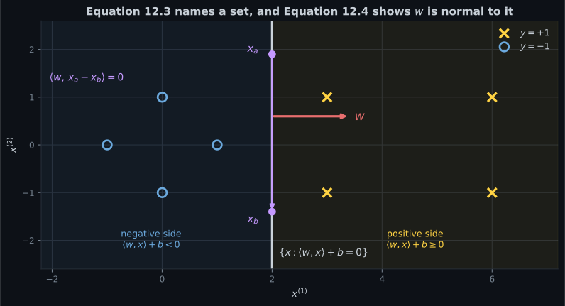
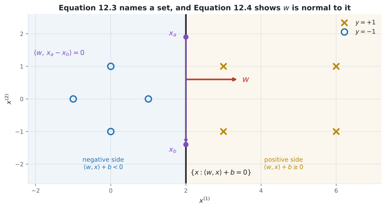
The two classes are separated by the vertical line $x^{(1)} = 2$. The nearest positive points are $(3, \pm 1)$ and the nearest negative point is $(1, 0)$, so the gap between the classes is exactly $2$ and the maximum margin is exactly $1$. Under the scaling Section 12.2.2 adopts this makes $\mathbf{w}^* = (1, 0)$ and $b^* = -2$, with $\lVert\mathbf{w}^*\rVert = 1$.

check_the_answer.py

from scipy.optimize import minimize
 
margins = Y * (X @ W_STAR + B_STAR)
print(f"y_n(<w*,x_n> + b*) : {margins}")
print(f"min over n         : {margins.min():.10f}")
print(f"||w*||             : {np.linalg.norm(W_STAR):.10f}")
print(f"support vectors    : {list(np.where(np.isclose(margins, 1))[0])}")
 
# and solve (12.18)-(12.19) numerically, to be sure
res = minimize(lambda v: 0.5 * v[:2] @ v[:2], np.array([0.3, 0.3, 0.0]),
               constraints=[{"type": "ineq",
                             "fun": lambda v: Y * (X @ v[:2] + v[2]) - 1}],
               method="SLSQP", options={"maxiter": 2000, "ftol": 1e-14})
print(f"SLSQP w = {np.round(res.x[:2], 10)}, b = {res.x[2]:.10f}")
print(f"largest deviation  : "
      f"{max(np.abs(res.x[:2] - W_STAR).max(), abs(res.x[2] - B_STAR)):.3e}")

text

y_n(<w*,x_n> + b*) : [1. 1. 4. 4. 1. 2. 2. 3.]
min over n         : 1.0000000000
||w*||             : 1.0000000000
support vectors    : [0, 1, 4]
SLSQP w = [ 1. -0.], b = -2.0000000000
largest deviation  : 3.997e-15

Three of the eight points sit exactly on the margin and five do not. That split is the whole subject of page 1206.

Why w is normal to the hyperplane

The book’s argument is four lines and worth following, because it is the only place in the chapter where the geometry is proved rather than asserted. Take any two points $\mathbf{x}_a$, $\mathbf{x}_b$ on the hyperplane. Then

$$f(\mathbf{x}_a) - f(\mathbf{x}_b) = \langle\mathbf{w}, \mathbf{x}_a\rangle + b - (\langle\mathbf{w}, \mathbf{x}_b\rangle + b) = \langle\mathbf{w}, \mathbf{x}_a - \mathbf{x}_b\rangle \qquad \text{(12.4a), (12.4b)}$$

and since both points are on the hyperplane, both values are zero, so $\langle\mathbf{w}, \mathbf{x}_a - \mathbf{x}_b\rangle = 0$. Every vector lying in the hyperplane is orthogonal to $\mathbf{w}$. The intercept $b$ never appears in the conclusion — it cancels in the first step — which is why $\mathbf{w}$ alone fixes the orientation and $b$ alone fixes the position.

w_is_normal.py

rng = np.random.default_rng(0)
worst = 0.0
for _ in range(200000):
    t1, t2 = rng.normal(0, 50, 2)          # two points on x = 2
    p1, p2 = np.array([2.0, t1]), np.array([2.0, t2])
    worst = max(worst, abs(W_STAR @ (p1 - p2)))
print(f"worst |<w, x_a - x_b>| over 200,000 random pairs : {worst:.3e}")

text

worst |<w, x_a - x_b>| over 200,000 random pairs : 0.000e+00

Exactly zero, not nearly zero — because the difference vector is $(0, t_1 - t_2)$ and $\mathbf{w}$ is $(1, 0)$, so the product of the only surviving term is $0 \times (t_1-t_2)$.

figure Equation 12.3 names a set, and Equation 12.4 shows w is normal to it matplotlib

The purple vector lies in the hyperplane and the red one is orthogonal to it. Note that the labels 'positive side' and 'negative side' come from Equations 12.5 and 12.6, not from Equation 12.3 — the set alone does not say which side is which.

A hyperplane is a set; (w, b) is not

Equation 12.3 defines the classifier as a set, and a set does not determine the parameters that name it. Every positive multiple of $(\mathbf{w}, b)$ gives the same set and the same predictions:

scale_invariance.py

base = np.sign(X @ W_STAR + B_STAR)
print(f"{'c':>8} {'w':>16} {'b':>9} {'same labels?':>14}")
for c in (0.5, 1.0, 2.0, 17.0, 1000.0):
    w2, b2 = c * W_STAR, c * B_STAR
    same = bool((np.sign(X @ w2 + b2) == base).all())
    print(f"{c:>8.1f} {str(np.round(w2, 1)):>16} {b2:>9.1f} {str(same):>14}")

text

       c                w         b   same labels?
     0.5        [0.5 0. ]      -1.0           True
     1.0          [1. 0.]      -2.0           True
     2.0          [2. 0.]      -4.0           True
    17.0        [17.  0.]     -34.0           True
  1000.0    [1000.    0.]   -2000.0           True

So “the distance from a point to the hyperplane” has no meaning until a scale is fixed. The value $f(\mathbf{x}) = \langle\mathbf{w},\mathbf{x}\rangle + b$ can be made as large or as small as you like without moving anything. This one-parameter freedom is the “technical wrinkle” §12.2.1 opens with, and Sections 12.2.1 and 12.2.2 are two different ways of spending it: fix $\lVert\mathbf{w}\rVert = 1$, or fix the value at the closest point to $1$.

Equations 12.5, 12.6 and 12.7 are not quite equivalent

The book writes the two conditions for correct classification

$$\langle\mathbf{w},\mathbf{x}_n\rangle + b \geq 0 \ \text{ when } y_n = +1, \qquad \langle\mathbf{w},\mathbf{x}_n\rangle + b < 0 \ \text{ when } y_n = -1 \qquad \text{(12.5), (12.6)}$$

and then combines them:

$$y_n(\langle\mathbf{w},\mathbf{x}_n\rangle + b) \geq 0 \qquad \text{(12.7)}$$

saying “Equation (12.7) is equivalent to (12.5) and (12.6) when we multiply both sides of (12.5) and (12.6) with $y_n = 1$ and $y_n = -1$, respectively.”

Multiplying an inequality by $-1$ reverses it, so 12.6’s strict $<$ becomes a strict $>$, and 12.7 should read $y_n f(\mathbf{x}_n) > 0$ for the negative class. As printed, the two are not the same condition:

the_boundary_case.py

z = np.array([2.0, 0.0])              # exactly ON the hyperplane
fz = W_STAR @ z + B_STAR
print(f"f(z) = {fz:.1f}, and suppose its label is y = -1")
print(f"  12.6 requires f(z) < 0    : {fz < 0}")
print(f"  12.7 requires y*f(z) >= 0 : {(-1.0) * fz >= 0}")

text

f(z) = 0.0, and suppose its label is y = -1
  12.6 requires f(z) < 0    : False
  12.7 requires y*f(z) >= 0 : True

Equation 12.7 admits a point that Equation 12.6 forbids. The disagreement is confined to the hyperplane itself, a set of measure zero, and it never matters again — from Equation 12.9 onwards every condition asks for a strictly positive margin, which excludes the boundary anyway. But the asymmetry in 12.5 and 12.6 is a real choice the book makes silently: a point sitting exactly on the decision boundary is classified $+1$, because $f(\mathbf{x}_{\text{test}}) \geq 0$ is the test the text gives. Ties go to the positive class.

The measurement that motivates the whole chapter

Figure 12.3 shows several green lines, all separating the data, with the caption “there are many linear classifiers that separate orange crosses from blue discs.” That is the problem Section 12.2 exists to solve. Here is how bad it actually is.

Method. Sample $400{,}000$ pairs $(\mathbf{w}, b)$ with $\lVert\mathbf{w}\rVert = 1$; keep the ones that separate all eight training points; score each survivor on $200{,}000$ held-out points drawn from two isotropic Gaussians centred at $(4.5, 0)$ and $(0, 0)$. Equal isotropic covariance means the Bayes-optimal rule is the perpendicular bisector of the two means, $x^{(1)} = 2.25$ — a known target to measure against.

how_many_separators.py

MU_POS, MU_NEG, SD, M = np.array([4.5, 0.0]), np.array([0.0, 0.0]), 1.0, 200000
rt = np.random.default_rng(7)
XT = np.vstack([rt.normal(MU_POS, SD, (M // 2, 2)),
                rt.normal(MU_NEG, SD, (M // 2, 2))])
YT = np.r_[np.ones(M // 2), -np.ones(M // 2)]
 
rg = np.random.default_rng(11)
accs, margins = [], []
for _ in range(400000):
    th = rg.uniform(0, 2 * np.pi)
    w, b = np.array([np.cos(th), np.sin(th)]), rg.uniform(-8, 8)
    if not (Y * (X @ w + b) > 0).all():      # must separate the training set
        continue
    accs.append(float((np.sign(XT @ w + b) == YT).mean()))
    margins.append(float((Y * (X @ w + b)).min()))
accs, margins = np.array(accs), np.array(margins)
 
print(f"separators found : {len(accs)} of 400,000")
print(f"held-out accuracy: worst {accs.min():.4f}  median "
      f"{np.median(accs):.4f}  best {accs.max():.4f}")
print(f"correlation(margin, accuracy) : {np.corrcoef(margins, accs)[0,1]:.6f}")
print(f"{'margin bin':>14} {'count':>7} {'mean acc':>10} {'worst acc':>10}")
edges = [0.0, 0.2, 0.4, 0.6, 0.8, 1.0]
for lo, hi in zip(edges[:-1], edges[1:]):
    m = (margins >= lo) & (margins < hi)
    print(f"  [{lo:.1f}, {hi:.1f})".rjust(14) + f" {int(m.sum()):>7} "
          f"{accs[m].mean():>10.4f} {accs[m].min():>10.4f}")

text

separators found : 9628 of 400,000
held-out accuracy: worst 0.8757  median 0.9662  best 0.9877
correlation(margin, accuracy) : 0.590999
    margin bin   count   mean acc  worst acc
    [0.0, 0.2)    2998     0.9381     0.8757
    [0.2, 0.4)    2630     0.9544     0.9037
    [0.4, 0.6)    2113     0.9685     0.9297
    [0.6, 0.8)    1349     0.9779     0.9606
    [0.8, 1.0)     538     0.9832     0.9777

Nine thousand six hundred and twenty-eight classifiers, all with zero training error, and their held-out accuracy spans $0.1119$. Empirical risk on the training set cannot tell them apart — every one of them scores perfectly. Something else has to choose, and the table says what.

figure Zero training error does not pick a classifier — Figure 12.3, measured matplotlib

The red curve is the finding. The best accuracy in each bin barely moves — the top edge of the scatter is almost flat — while the worst rises from 0.8757 to 0.9777. A large margin does not promise the best classifier; it rules out the bad ones.

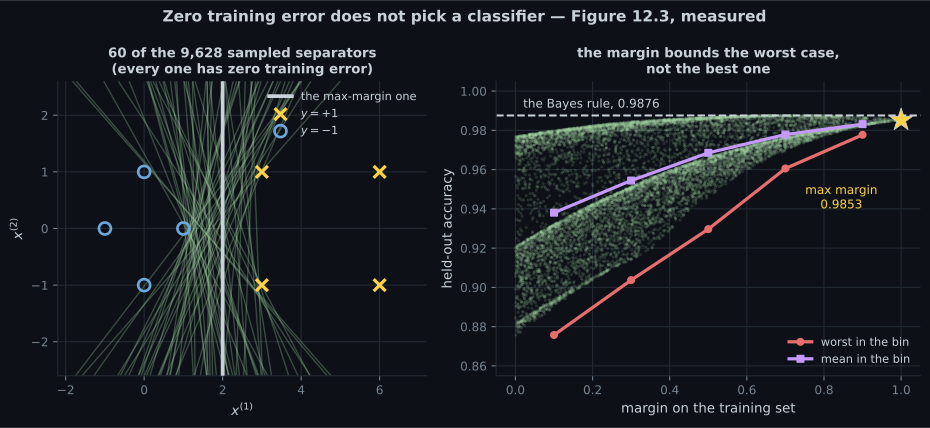
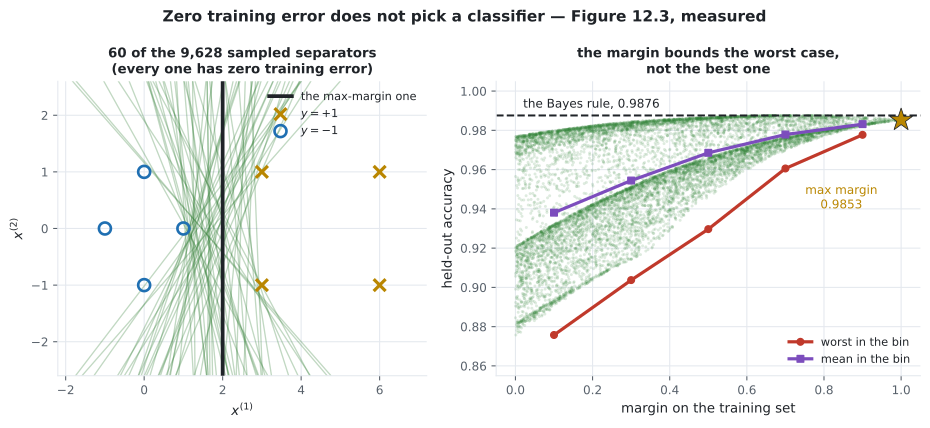
The margin bounds the worst case, not the best one. That distinction is worth being precise about, because it is easy to overclaim:

claim	true?	measured
larger margin correlates with better held-out accuracy	yes	$r = 0.590999$
the maximum-margin separator beats most others	yes	it beats $91.76\%$ of the $9{,}628$
the maximum-margin separator is the best of them	no	best sampled $0.9877$ vs its $0.9853$
the maximum-margin separator is Bayes-optimal	no	Bayes $0.9876$ at $x = 2.25$, SVM at $x = 2.00$

The best separator found scores $0.9877$ — essentially the Bayes rate — at a margin of only $0.756759$. It got there by luck, and nothing on the training set could have identified it. The maximum-margin rule gives up $0.0024$ against that lucky draw in exchange for never landing in the $0.8757$ tail.

Why the margin is not Bayes-optimal here, and why that is fine

The SVM’s boundary sits at $x^{(1)} = 2.00$ because the training set’s nearest points are at $x = 1$ and $x = 3$. The Bayes boundary sits at $x^{(1)} = 2.25$ because the class means are at $0$ and $4.5$. The SVM is looking at the closest examples and the Bayes rule at the whole distribution — with eight points, the closest examples are a noisy estimate of where the classes end.

This is the trade the book points at when it cites Steinwart and Christmann (2008) in the margin note “a classifier with large margin turns out to generalize well.” What those results bound is the generalisation gap, not the error itself. The $0.0023$ shortfall against Bayes is what eight points cost; the $0.1119$ spread is what having no principle at all would cost.

pch.quizTag Check your understanding

1. A They are uniquely determined by the set B Only w is determined; b is free C Every positive multiple of (w, b) names the same set and the same classifier, so the pair is determined only up to a positive scale D The set determines w up to sign only
   pch.quizShowAnswer

   C — Every positive multiple of (w, b) names the same set and the same classifier, so the pair is determined only up to a positive scale

2. A Because b is assumed to be zero B Because it cancels when subtracting f(x_b) from f(x_a) — which is why w alone fixes the hyperplane's orientation and b alone its position C Because x_a and x_b are orthogonal D Because the inner product is linear in b
   pch.quizShowAnswer

   B — Because it cancels when subtracting f(x_b) from f(x_a) — which is why w alone fixes the hyperplane's orientation and b alone its position

3. A Nowhere; they are equivalent B For points far from the hyperplane C On the hyperplane itself: 12.6 is strict, so multiplying by -1 should give a strict inequality, but 12.7 is written with >=. A point with f(z) = 0 and label -1 satisfies 12.7 and violates 12.6 D When the labels are 0 and 1 rather than plus and minus one
   pch.quizShowAnswer

   C — On the hyperplane itself: 12.6 is strict, so multiplying by -1 should give a strict inequality, but 12.7 is written with >=. A point with f(z) = 0 and label -1 satisfies 12.7 and violates 12.6

4. A The highest possible held-out accuracy B A guarantee of Bayes optimality C A raised floor: the worst accuracy per margin bin climbs from 0.8757 to 0.9777 while the best barely moves. The max-margin solution beats 91.76 percent of them but is not the best D Nothing measurable; the correlation is zero
   pch.quizShowAnswer

   C — A raised floor: the worst accuracy per margin bin climbs from 0.8757 to 0.9777 while the best barely moves. The max-margin solution beats 91.76 percent of them but is not the best

Exercises

Exercise 1 – Show that w is normal to the hyperplane

pch.exerciseTag pch.exerciseTitle

Exercise 2 – Rescale the parameters and find nothing changes

pch.exerciseTag pch.exerciseTitle

Exercise 3 – Count the separators, and score them

pch.exerciseTag pch.exerciseTitle

Recall card

• Chapter 12 is the last of the four pillars, classification, and it reasons geometrically rather than probabilistically — closer to Chapter 10’s derivation of PCA than to Chapter 9’s likelihood.
• The chapter prints no numbers at all. It has no worked examples, so every value on these pages is this module’s own, computed on an eight-point running example whose answer is exact.
• A hyperplane is the zero set of an affine function, and the classifier is the sign of that function.
• w is normal to the hyperplane, proved by subtracting the function’s value at two points on it. The intercept cancels in that subtraction, which is why w fixes the orientation and b fixes the position.
• The set does not determine the parameters. Every positive multiple of w and b names the same classifier, so the raw value of f carries no notion of distance until a scale is chosen.
• That freedom is spent twice in Section 12.2, once by demanding a unit-length w and once by demanding the value one at the closest point — and page 1203 shows the two agree.
• Equations 12.5 and 12.6 are not symmetric. One is inclusive and one is strict, so ties on the boundary go to the positive class, and the combined Equation 12.7 is very slightly weaker than the pair it replaces.
• Zero training error does not pick a classifier. 9,628 sampled hyperplanes separate the eight points perfectly and their held-out accuracy spans 0.1119.
• Margin and held-out accuracy correlate at 0.590999, and the maximum-margin solution beats 91.76 percent of those separators.
• But it is not the best of them, scoring 0.9853 against a best sampled 0.9877 and a Bayes rate of 0.9876. The margin raises the floor — the worst case per bin climbs from 0.8757 to 0.9777 — while the ceiling barely moves.
• So maximising the margin is insurance rather than optimisation, which is exactly what the generalisation bounds the book cites actually prove.

Next: The Concept of the Margin — §12.2.1, and the wrinkle that a distance needs a scale.