
Phase 3 - Computer Vision with CNNs
Convolution exists because a Dense layer is the wrong shape for an image. On a
224×224×3 photograph, Dense(32) costs 4,816,928 parameters; a Conv2D(32, 3)
costs 896 — and unlike the dense layer, that number does not change when the image
does. Everything in this phase follows from weight sharing and locality.
Every number on these ten pages was measured on this machine, on a CPU, and the measurements are reproducible in minutes. Where a result contradicted the textbook claim, the page says so.
The pages
Section titled “The pages”| # | Page | The measured headline |
|---|---|---|
| 421 | Intro to CNNs | 896 parameters against 4,816,928; convolution matched TensorFlow at 2.38e-07; two 3×3 layers beat one 5×5 (18 weights against 25) |
| 422 | Pooling & CNN Architecture | average 0.8740, max 0.8720, strided convolution last at 0.8455; Flatten→Dense held 803,072 of 880,936 weight bytes |
| 423 | Famous Architectures | VGG-ish 0.8800 wins; plain beat residual at 12 convolutions (0.8500 vs 0.8433) |
| 423.5 | Normalisation Beyond Batch | layer norm won at batches 4/16/64, batch norm overtook it at 256 — exactly where the statistic counts cross |
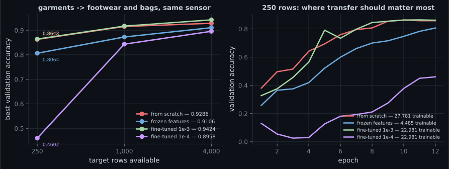
| 424 | Transfer Learning | fine-tuning beat scratch by +0.0014, freezing lost at every size, and a wrong learning rate cost 0.4026 |
| 424.5 | Fine-Tuning and LoRA | LoRA reached 0.8911 training 2.80% of the weights against full fine-tuning’s 0.9385 — and training from scratch beat both at 0.9350 |
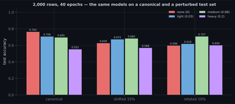
| 425 | Data Augmentation | cost 0.1855 on canonical data and bought 0.1105 on rotated data — invariance, not accuracy |
| 426 | Image Segmentation | pixel accuracy 0.9737 against a do-nothing baseline of 0.8691; report IoU |
| 427 | Interpreting Convnets | activations grow 1.61 → 20.44 with depth; 4 of 64 channels silent; always run the random-weights check |
| 428 | Object Detection | 32.8 : 1 cell imbalance; recall 0.8616 → 0.6799 while precision sat at 0.997 |
| 428.5 | Vision Transformers | the ViT beat the convnet at 1,000 and 4,000 rows — and overfitted 4× harder |
  flowchart TD
  A["421 Convolution
weight sharing, receptive field"] --> B["422 Pooling & the stack
downsampling, memory"]
  B --> C["423 Famous architectures
LeNet to Xception"]
  C --> D["423.5 Normalisation
batch, layer, group, instance"]
  D --> E["424 Transfer learning
freeze, fine-tune, probe"]
  E --> L["424.5 LoRA
low-rank adaptation"]
  L --> F["425 Augmentation
invariance, not accuracy"]
  F --> G["426 Segmentation
per-pixel labels, IoU"]
  G --> H["427 Interpretation
activations, Grad-CAM"]
  H --> I["428 Detection
grids, IoU, NMS"]
  I --> J["428.5 Vision transformers
patches and attention"]
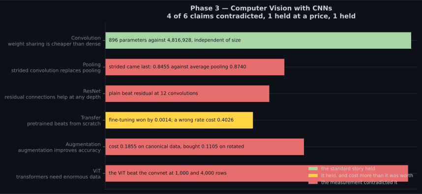
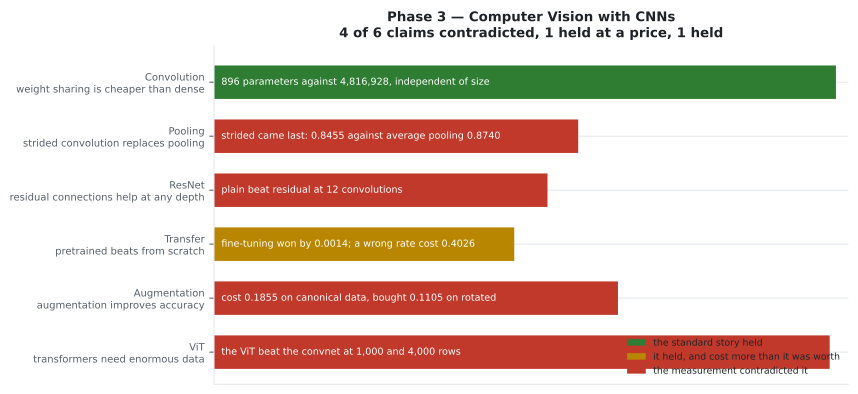
Four results that contradict the usual story
Section titled “Four results that contradict the usual story”Each of these is measured on this data, at this scale — which is exactly the caveat that makes them useful rather than misleading.
- Strided convolution came last. The “learnable downsampling replaces pooling” advice lost to plain average pooling by 0.0285. A fixed rule with no parameters beat a learned one at equal capacity.
- Plain convolutions beat residual ones at 12 layers. Residual connections solve a problem that starts at depths this phase cannot afford; at 12 convolutions they cost 0.0067. Their direction was still visible — depth helped the residual family eight times more.
- Augmentation hurt at every dataset size. Fashion-MNIST is centred and pose-normalised, and the un-augmented model was not overfitting. Augmentation encodes an invariance assumption; if the test set has no such variance, it is pure cost.
- The ViT beat the convnet at 1,000 rows. “Transformers need enormous data” is a claim about 196+ tokens on 224×224 photographs. At 16 tokens on centred 28×28 greyscale, the convolutional prior is worth very little.
Three mistakes that were mine, and are now on the pages
Section titled “Three mistakes that were mine, and are now on the pages”Every one of these produced a plausible-looking number before it was caught.
- Batch normalisation’s default momentum of 0.99 needs roughly 460 batches for its moving averages to settle. A 376-batch run reported validation accuracy of 0.1540 with a training loss of 0.27. Lowering it to 0.9 fixed it, and the incident is written up on page 423.
- A ReLU placed before the
Addin a residual block made the residual model worse than the plain one, because activations then grow additively with depth. The classic ordering is conv-BN-relu-conv-BN →Add→ relu. - A fixed epoch budget measured the budget rather than the treatment: augmented runs were still climbing at epoch 15 while plain runs had stopped. Page 425 reports the best epoch per run for exactly this reason.
What carries into the rest of the module
Section titled “What carries into the rest of the module”| Idea from this phase | Where it comes back |
|---|---|
| weight sharing over a structured axis | 1D convolution over time, Phase 4 |
| layer normalisation, no batch statistics | every transformer block, Phases 4–6 |
| residual connections around a sublayer | transformer blocks, diffusion U-Nets |
| the encoder–decoder hourglass with skips | U-Net diffusion models, Phase 6 |
| attention over a set of tokens | the whole of Phase 5 |
| “compare against the do-nothing baseline” | forecasting, detection, generation |
-
On 224x224x3 input, `Dense(32)` costs 4,816,928 parameters and `Conv2D(32, 3)` costs 896. Which part of that comparison matters most?
pch.quizShowAnswer
B — That the convolution's count does not depend on the image size at all, because the same 3x3 kernel is reused at every position
-
Augmentation cost 0.1855 on canonical test data and bought 0.1105 on rotated test data. What is the correct conclusion?
pch.quizShowAnswer
B — Augmentation encodes an invariance assumption, so it pays exactly when the deployment distribution contains that variance and costs accuracy when it does not
-
Fine-tuning at learning rate 1e-4 reached only 0.4602 at 250 rows while 1e-3 reached 0.8642. Why is the low-rate result NOT evidence against fine-tuning?
pch.quizShowAnswer
B — Because the per-epoch curve shows it was still climbing at epoch 12 - it is a budget mismatch, not a property of the method
-
Batch normalisation's default momentum of 0.99 needs roughly 460 batches to settle, and a 376-batch run reported validation accuracy of 0.1540 with a training loss of 0.27. What was actually broken?
pch.quizShowAnswer
B — Nothing in the model - the moving averages used at inference time had not converged, so training and validation were effectively using different normalisation statistics
-
A vision transformer BEAT the convnet at 1,000 and 4,000 rows, contradicting 'transformers need enormous data'. What makes both statements true at once?
pch.quizShowAnswer
B — The usual claim is about 196+ tokens on 224x224 photographs; at 16 tokens on centred 28x28 greyscale, the convolutional prior is worth very little, so there is far less for the transformer to relearn
pch.coffeeTagline
pch.coffeeCtapch.feedbackHeading
pch.feedbackSubheading