What you’ll learn

• what separates a regression problem from a classification problem
• the general linear model $\hat{y} = \boldsymbol{\theta}^\top \mathbf{x}$, and why the bias term gets folded into the feature vector
• the two ways to fit it — closed form and iterative — and when each wins
• how to compute a baseline first, and why a model that cannot beat it is worthless
• the assumptions behind linear regression, in the order you should check them
• the vocabulary the rest of Phase 3 relies on

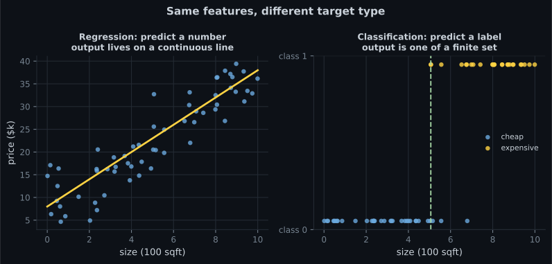
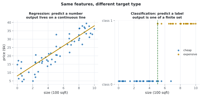
Intuition

Regression answers how much, not which one. How much will this house sell for, how many units will ship next quarter, how many days until this machine fails. The answer is a number on a continuous scale, and being close counts — predicting 302 when the truth is 300 is nearly right, in a way that predicting “cat” when the truth is “dog” never is.

That single difference drives everything: the loss functions, the metrics, even the plots.

figureSame features, different target typematplotlib

  flowchart LR
  D["Raw data"] --> F["Feature vector x"]
  F --> M["Model with parameters theta"]
  M --> P["Prediction ŷ (a number)"]
  P --> C["Cost: how wrong, on average"]
  T["True target y"] --> C
  C -->|"adjust theta"| M

The math

The general linear model

With $n$ features, a linear model computes a weighted sum plus a bias:

Carrying that leading $\theta_0$ around separately is a nuisance, so by convention we prepend a constant feature $x_0 = 1$ to every instance. The model collapses into a dot product:

For a whole dataset of $m$ instances stacked into a matrix $\mathbf{X} \in \mathbb{R}^{m \times (n+1)}$, all predictions at once are one matrix-vector product:

Training means choosing $\boldsymbol{\theta}$

Fitting is a search for the parameter vector that makes a cost function smallest. Almost always that cost is mean squared error:

There are exactly two routes to the minimum, and Phase 3 covers both:

  flowchart LR
  T["Find theta minimising J"] --> N["Normal Equation
closed form, one shot"]
  T --> G["Gradient Descent
iterative, many small steps"]
  N --> S["The same theta"]
  G --> S

Worked example by hand

Three houses, two features. Price in thousands, size in hundreds of square feet:

Suppose a model arrives with $\boldsymbol{\theta} = [50,\ 6,\ 18]^\top$ — a base price of 50, six thousand per hundred square feet, eighteen thousand per bedroom.

Predictions. Each one is a dot product:

Errors.

So this $\boldsymbol{\theta}$ is off by about 23,800 on a typical house — and it under-predicts more as houses get bigger, which is the tell that the size coefficient is too small. Training is the process of finding the $\boldsymbol{\theta}$ that drives $J$ as low as it will go.

See it move

Each bar below is one term of the weighted sum. Watch them accumulate left to right into the final prediction — that is all a linear model does at inference time.

From scratch

The hypothesis function is four lines of NumPy:

import numpy as np
 
 
def add_bias(X):
    """Prepend the x0 = 1 column so the bias rides inside the dot product."""
    X = np.asarray(X, dtype=float)
    return np.c_[np.ones(len(X)), X]
 
 
def predict(X_with_bias, theta):
    """All m predictions at once: one matrix-vector product."""
    return X_with_bias @ theta
 
 
X = [[10, 2], [15, 3], [20, 4]]        # size (100 sqft), bedrooms
y = np.array([145.0, 210.0, 280.0])
theta = np.array([50.0, 6.0, 18.0])    # bias, w_size, w_beds
 
Xb = add_bias(X)
print(Xb)
# [[ 1. 10.  2.]
#  [ 1. 15.  3.]
#  [ 1. 20.  4.]]
 
pred = predict(Xb, theta)
print(pred)                                             # [146. 194. 242.]
print(f"MSE  = {((pred - y) ** 2).mean():.1f}")         # MSE  = 567.0
print(f"RMSE = {((pred - y) ** 2).mean() ** 0.5:.1f}")  # RMSE = 23.8

import numpy as np
 
 
def add_bias(X):
    """Prepend the x0 = 1 column so the bias rides inside the dot product."""
    X = np.asarray(X, dtype=float)
    return np.c_[np.ones(len(X)), X]
 
 
def predict(X_with_bias, theta):
    """All m predictions at once: one matrix-vector product."""
    return X_with_bias @ theta
 
 
X = [[10, 2], [15, 3], [20, 4]]        # size (100 sqft), bedrooms
y = np.array([145.0, 210.0, 280.0])
theta = np.array([50.0, 6.0, 18.0])    # bias, w_size, w_beds
 
Xb = add_bias(X)
print(Xb)
# [[ 1. 10.  2.]
#  [ 1. 15.  3.]
#  [ 1. 20.  4.]]
 
pred = predict(Xb, theta)
print(pred)                                             # [146. 194. 242.]
print(f"MSE  = {((pred - y) ** 2).mean():.1f}")         # MSE  = 567.0
print(f"RMSE = {((pred - y) ** 2).mean() ** 0.5:.1f}")  # RMSE = 23.8

Exactly the hand calculation, to the digit.

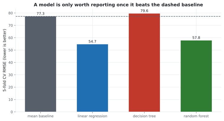
Baselines matter

Before any model, compute the score of the laziest possible predictor. For regression that is “always predict the mean of the training targets”. Everything else has to beat it, and it is startling how often something does not:

from sklearn.datasets import load_diabetes
from sklearn.dummy import DummyRegressor
from sklearn.linear_model import LinearRegression
from sklearn.tree import DecisionTreeRegressor
from sklearn.ensemble import RandomForestRegressor
from sklearn.model_selection import cross_val_score
 
X, y = load_diabetes(return_X_y=True)
 
models = {
    "mean baseline": DummyRegressor(strategy="mean"),
    "linear regression": LinearRegression(),
    "decision tree": DecisionTreeRegressor(random_state=0),
    "random forest": RandomForestRegressor(n_estimators=120, random_state=0),
}
 
for name, model in models.items():
    rmse = -cross_val_score(
        model, X, y, cv=5, scoring="neg_root_mean_squared_error"
    ).mean()
    print(f"{name:<20} RMSE = {rmse:6.2f}")
 
# mean baseline        RMSE =  77.26
# linear regression    RMSE =  54.69
# decision tree        RMSE =  79.55
# random forest        RMSE =  57.79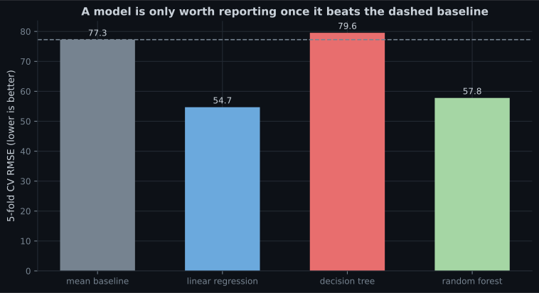

from sklearn.datasets import load_diabetes
from sklearn.dummy import DummyRegressor
from sklearn.linear_model import LinearRegression
from sklearn.tree import DecisionTreeRegressor
from sklearn.ensemble import RandomForestRegressor
from sklearn.model_selection import cross_val_score
 
X, y = load_diabetes(return_X_y=True)
 
models = {
    "mean baseline": DummyRegressor(strategy="mean"),
    "linear regression": LinearRegression(),
    "decision tree": DecisionTreeRegressor(random_state=0),
    "random forest": RandomForestRegressor(n_estimators=120, random_state=0),
}
 
for name, model in models.items():
    rmse = -cross_val_score(
        model, X, y, cv=5, scoring="neg_root_mean_squared_error"
    ).mean()
    print(f"{name:<20} RMSE = {rmse:6.2f}")
 
# mean baseline        RMSE =  77.26
# linear regression    RMSE =  54.69
# decision tree        RMSE =  79.55
# random forest        RMSE =  57.79

figureFour models against the same baselinematplotlib

Reading the plot

• Linear regression wins. On 442 samples with ten mostly-linear features, the simplest model is also the best. That is common, and worth internalising early.
• The lone decision tree loses to the baseline. It memorises the training set and generalises worse than a constant. Without a baseline you would never notice.
• The forest recovers most of the gap but still loses. Extra capacity has to be paid for with signal that actually exists in the data.

Assumptions, in checking order

Note the wording of the first row: linear in the parameters, not in the features. $\hat{y} = \theta_0 + \theta_1 x + \theta_2 x^2$ is still a linear model — it is linear in $\boldsymbol{\theta}$, and that is what lets the same math fit a curve. Polynomial Regression is built entirely on that loophole.

Where regression shows up

Pitfalls

🧪 Try It Yourself

Exercise 1 – Build the feature vector

Exercise 2 – Predict with the hypothesis function

Exercise 3 – Score the parameters

Exercise 4 – Beat the mean baseline

Exercise 5 – A curve, still fitted by a linear model

Recap

• Regression predicts a continuous number; closeness counts, which shapes every loss and metric.
• Folding $x_0 = 1$ into the feature vector turns the model into a single dot product $\hat{y} = \boldsymbol{\theta}^\top\mathbf{x}$.
• Training means minimising a cost — via the Normal Equation for modest feature counts, via gradient descent for large ones.
• Always compute the mean baseline. On the diabetes data it is RMSE 77.26; linear regression reaches 54.69 while a single decision tree manages only 79.55.
• “Linear” describes the parameters, not the shape of the curve.

Exercise 6 – Price each model against the baseline

Next

Continue to Simple Linear Regression — the one-feature case, derived from scratch and worked through by hand on five points.