Affine Spaces

Everything so far insisted on passing through the origin. Subspaces must contain $\mathbf{0}$; linear mappings must send $\mathbf{0}$ to $\mathbf{0}$. That insistence bought a great deal of structure, and it also excluded most of the objects you actually care about: a regression line with a nonzero intercept, a decision boundary that is not through the origin, a neural network layer with a bias.

This section relaxes it, in the smallest possible way: take a subspace and slide it.

What you’ll learn

• What an affine subspace is — support point plus direction space — and why it is not a subspace.
• The parametric equation, and why the representation is unique once you fix an ordered basis.
• Lines, planes and hyperplanes, and the dimension counting behind each.
• Why the solution set of an inhomogeneous system is exactly an affine subspace.
• Affine mappings, and the fact that every one is a linear mapping followed by a translation.

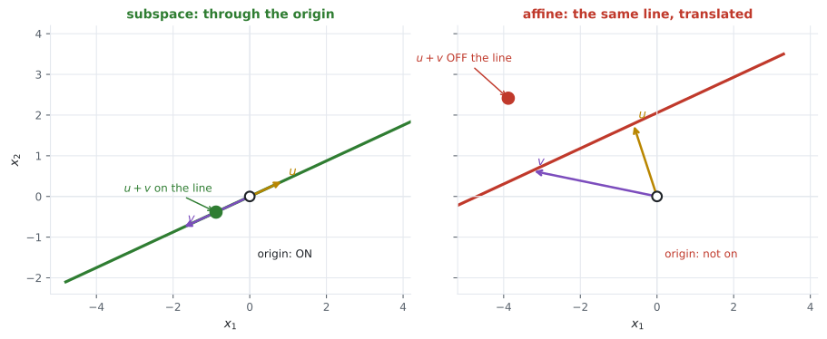
Intuition: a regression line

Fit a straight line to data and you get $y = wx + b$. If $b \neq 0$ the line does not pass through the origin, so the set of points on it is not a subspace. It fails the very first test: the origin is not on it.

But it is only barely not a subspace. Take the line $y = wx$ through the origin — that is a subspace, a one-dimensional one — and slide it up by $b$. Same direction, shifted position. That is the entire construction, and the terminology follows it:

• the direction space is the subspace you started with,
• the support point is how far you slid it.

diagram Diagram mermaid

  flowchart TD
  S["a subspace U
contains 0, closed"] --> T["slide it by x0"]
  T --> L["AFFINE SUBSPACE
L = x0 + U"]
  L --> N1["contains 0 only if x0 is in U
-> otherwise NOT a subspace"]
  L --> N2["not closed under addition or scaling"]
  L --> P["parametric equation
x = x0 + lambda1 b1 + ... + lambdak bk"]
  P --> D1["k = 1: a LINE"]
  P --> D2["k = 2: a PLANE"]
  P --> D3["k = n-1: a HYPERPLANE"]
  L --> SOL["the solution set of Ax = b
is exactly one of these"]

The math

Affine subspace

Let $V$ be a vector space, $\mathbf{x}_0 \in V$, and $U \subseteq V$ a subspace. The subset

$$L = \mathbf{x}_0 + U := \{\mathbf{x}_0 + \mathbf{u} : \mathbf{u} \in U\} = \{\mathbf{v} \in V : \exists\mathbf{u} \in U,\; \mathbf{v} = \mathbf{x}_0 + \mathbf{u}\} \subseteq V$$

is an affine subspace of $V$, also called a linear manifold. $U$ is the direction or direction space, and $\mathbf{x}_0$ is the support point.

The definition excludes $\mathbf{0}$ whenever $\mathbf{x}_0 \notin U$. So an affine subspace is not a linear subspace in that case — the book says so explicitly, and it is the whole distinction.

Neither the support point nor the parameters are canonical

Any point of $L$ works as the support point. Slide the line $y = 2x + 1$ from $(0,1)$ or from $(1,3)$ — same line. So “the support point” is not a well-defined phrase without a choice.

The book gives the precise containment test that goes with this: for $L = \mathbf{x}_0 + U$ and $\tilde{L} = \tilde{\mathbf{x}}_0 + \tilde{U}$,

$$L \subseteq \tilde{L} \iff U \subseteq \tilde{U} \text{ and } \mathbf{x}_0 - \tilde{\mathbf{x}}_0 \in \tilde{U}$$

Two conditions: the directions nest, and the offset between support points is itself a direction. The second is what makes the test about the sets rather than the arbitrary choices.

The parametric equation

If $L = \mathbf{x}_0 + U$ is $k$-dimensional and $(\mathbf{b}_1,\dots,\mathbf{b}_k)$ is an ordered basis of $U$, then every $\mathbf{x} \in L$ can be uniquely described as

$$\mathbf{x} = \mathbf{x}_0 + \lambda_1\mathbf{b}_1 + \cdots + \lambda_k\mathbf{b}_k$$

with $\lambda_1,\dots,\lambda_k \in \mathbb{R}$. This is the parametric equation of $L$ with directional vectors $\mathbf{b}_1,\dots,\mathbf{b}_k$ and parameters $\lambda_1,\dots,\lambda_k$.

Uniqueness here is §2.6’s uniqueness-of-coordinates, inherited: once $\mathbf{x}_0$ and the ordered basis are fixed, the parameters are determined. Change the support point and every $\lambda$ shifts, but for a given choice there is exactly one answer.

Lines, planes, hyperplanes

$k$	name	parametric equation	in $\mathbb{R}^n$
1	line	$\mathbf{y} = \mathbf{x}_0 + \lambda\mathbf{x}_1$	needs a support point and 1 direction
2	plane	$\mathbf{y} = \mathbf{x}_0 + \lambda_1\mathbf{x}_1 + \lambda_2\mathbf{x}_2$	2 linearly independent directions
$n-1$	hyperplane	$\mathbf{y} = \mathbf{x}_0 + \sum_{i=1}^{n-1}\lambda_i\mathbf{x}_i$	$n-1$ independent directions

The hyperplane row is the one worth internalising, because “hyperplane” is used constantly in machine learning and its dimension is relative:

• In $\mathbb{R}^2$, a hyperplane is a line.
• In $\mathbb{R}^3$, a hyperplane is a plane.
• In $\mathbb{R}^{1000}$, a hyperplane is a 999-dimensional object nobody can picture.

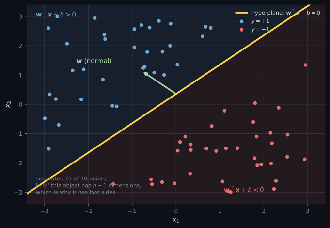
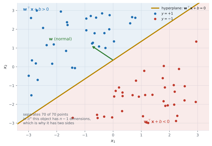
A hyperplane is always one dimension short of the ambient space, which is exactly why it divides it into two halves. That is what makes it a decision boundary, and Chapter 12 builds support vector machines on precisely this — the book even notes in this section that Chapter 12 will refer to such a subspace as a hyperplane.

Inhomogeneous systems are affine subspaces

The connection that makes this section retroactively explain §2.3. For $\mathbf{A} \in \mathbb{R}^{m\times n}$ and $\mathbf{b} \in \mathbb{R}^m$, the solution set of $\mathbf{A}\mathbf{x} = \mathbf{b}$ is either empty or an affine subspace of $\mathbb{R}^n$ of dimension $n - \operatorname{rk}(\mathbf{A})$.

That is §2.3’s particular-plus-general decomposition, renamed:

$$\underbrace{\mathbf{x}_p}_{\text{support point}} + \underbrace{\ker(\mathbf{A})}_{\text{direction space}}$$

And the converse holds too: in $\mathbb{R}^n$, every $k$-dimensional affine subspace is the solution of an inhomogeneous system $\mathbf{A}\mathbf{x} = \mathbf{b}$ with $\operatorname{rk}(\mathbf{A}) = n - k$. Affine subspaces and inhomogeneous systems are two descriptions of one thing, exactly as subspaces and homogeneous systems were in §2.4.

Two special cases worth naming:

• The solution of a single equation $\lambda_1x_1 + \cdots + \lambda_nx_n = b$ with not all $\lambda_i$ zero is a hyperplane in $\mathbb{R}^n$. One equation removes one dimension.
• A homogeneous system’s solution set is a subspace, which the book notes can be thought of as “a special affine space with support point $\mathbf{x}_0 = \mathbf{0}$”.

So subspaces are affine subspaces that happen to be centred. The general notion is the affine one.

Affine mappings

For vector spaces $V, W$, a linear mapping $\Phi : V \to W$ and a vector $\mathbf{a} \in W$, the mapping

$$\phi : V \to W, \qquad \mathbf{x} \mapsto \mathbf{a} + \Phi(\mathbf{x})$$

is an affine mapping from $V$ to $W$, and $\mathbf{a}$ is the translation vector.

Three properties:

• Every affine mapping is the composition of a linear mapping and a translation: $\phi = \tau \circ \Phi$, and the two are uniquely determined.
• The composition $\phi' \circ \phi$ of affine mappings is affine.
• Affine mappings keep the geometric structure invariant, and preserve dimension and parallelism.

Every “linear layer” in deep learning is affine

A neural network layer computes $\mathbf{W}\mathbf{x} + \mathbf{b}$. That is an affine mapping, not a linear one — the bias $\mathbf{b}$ is the translation vector. It sends $\mathbf{0}$ to $\mathbf{b}$, not to $\mathbf{0}$, so §2.7’s definition rules it out.

The frameworks call these layers linear anyway (nn.Linear, Dense), and the terminology is entrenched. The book anticipates this in its opening remark: “in the machine learning literature, the distinction between linear and affine is sometimes not clear so that we can find references to affine spaces/mappings as linear spaces/mappings.”

There is also a standard trick worth knowing: append a constant $1$ to $\mathbf{x}$ and absorb $\mathbf{b}$ as an extra column of $\mathbf{W}$. The affine map in $\mathbb{R}^n$ becomes a genuinely linear map in $\mathbb{R}^{n+1}$. That is why design matrices in Chapter 9 carry a column of ones — it converts an affine fitting problem into a linear one, at the cost of one dimension.

Worked example by hand

A line in $\mathbb{R}^2$. Take $\mathbf{x}_0 = (-1.5, 1.4)^\top$ and direction $\mathbf{u} = (1.6, 0.7)^\top$. The parametric equation is $\mathbf{y} = \mathbf{x}_0 + \lambda\mathbf{u}$, so

$\lambda$	$\mathbf{y}$
$-2$	$(-4.7, 0.0)$
$-1$	$(-3.1, 0.7)$
$0$	$(-1.5, 1.4)$ — the support point
$1$	$(0.1, 2.1)$
$2$	$(1.7, 2.8)$

Is $\mathbf{0}$ on this line? We would need $\lambda$ with $-1.5 + 1.6\lambda = 0$ and $1.4 + 0.7\lambda = 0$, giving $\lambda = 0.9375$ and $\lambda = -2$ respectively. Different values, so no. The line misses the origin and is therefore not a subspace.

Closure fails, concretely. Take the two points at $\lambda = 0$ and $\lambda = 1$: $(-1.5, 1.4)$ and $(0.1, 2.1)$. Their sum is $(-1.4, 3.5)$. Is that on the line? Solve $-1.5 + 1.6\lambda = -1.4$, giving $\lambda = 0.0625$; then the second coordinate would be $1.4 + 0.7(0.0625) = 1.44375 \neq 3.5$. Not on the line. Affine subspaces are not closed under addition, which is the second reason they are not subspaces.

An inhomogeneous system, as an affine subspace. Solve $x_1 + x_2 + x_3 = 3$ in $\mathbb{R}^3$. One particular solution is $(3, 0, 0)$. The direction space is the null space of $[1, 1, 1]$, which is two-dimensional, spanned by $(1,-1,0)$ and $(1,0,-1)$. So

$$L = \begin{bmatrix}3\\0\\0\end{bmatrix} + \lambda_1\begin{bmatrix}1\\-1\\0\end{bmatrix} + \lambda_2\begin{bmatrix}1\\0\\-1\end{bmatrix}$$

Dimension $n - \operatorname{rk} = 3 - 1 = 2$: a plane in $\mathbb{R}^3$, which is also a hyperplane because $2 = 3 - 1$. Checking $\lambda_1 = 2, \lambda_2 = -1$: the point is $(3 + 2 - 1, -2, 1) = (4, -2, 1)$, and $4 - 2 + 1 = 3$ ✓.

And the affine-to-linear trick. The affine map $\phi(x) = 2x + 3$ on $\mathbb{R}$ becomes the linear map

$$\begin{bmatrix}2 & 3\end{bmatrix}\begin{bmatrix}x\\ 1\end{bmatrix} = 2x + 3$$

on $\mathbb{R}^2$. Check the zero test in the new space: the input $(0, 1)^\top$ is not the zero vector of $\mathbb{R}^2$, so nothing is violated — the trick works precisely because the augmented input never is zero.

See it move

The violet arrow is the support point; the amber arrow is the direction. The white point slides along the affine line as $\lambda$ changes. The dashed grey line is the direction space itself — parallel, and passing through the origin.

sketch A line as support point plus direction p5.js Pause Restart

The violet arrow is the support point x0. The amber arrow is the direction u. The point y = x0 + lambda*u (white) slides along the affine line (solid green) as lambda changes. The dashed grey line is the direction space U through the origin — parallel, but passing through 0.

The two lines are parallel and never meet. The grey one is a subspace — the origin sits on it. The green one is its translate, and no value of $\lambda$ ever brings the white point to the origin. That gap is the support point, and it is the whole difference between the two objects.

From scratch

affine_spaces.py

import numpy as np
 
# ---- a line as support point plus direction --------------------------
x0 = np.array([-1.5, 1.4])
u  = np.array([ 1.6, 0.7])
 
def on_line(y, tol=1e-9):
    """Is y on the affine line x0 + lambda*u? Solve both coordinates and compare."""
    lams = (y - x0) / u
    return np.allclose(lams, lams[0], atol=tol), lams
 
for lam in (-2.0, -1.0, 0.0, 1.0, 2.0):
    print(f"lambda={lam:5}  y = {x0 + lam * u}")
 
print("\nis the origin on the line?", on_line(np.zeros(2))[0],
      " -> the two lambdas disagree:", np.round(on_line(np.zeros(2))[1], 4))
 
# ---- affine subspaces are not closed --------------------------------
p, q = x0 + 0.0 * u, x0 + 1.0 * u
print("\ntwo points on the line:", p, q)
print("their sum:", p + q, " on the line?", on_line(p + q)[0])
print("2*p      :", 2 * p, "        on the line?", on_line(2 * p)[0])
print("-> not closed under addition OR scaling, so not a subspace")
 
# ---- but the DIRECTION space is a subspace --------------------------
d1, d2 = 1.3 * u, -0.4 * u
print("\ndirections", np.round(d1, 3), "and", np.round(d2, 3))
print("their sum is still a multiple of u:",
      np.allclose(np.cross(np.append(d1 + d2, 0), np.append(u, 0)), 0))
 
# ---- an inhomogeneous system IS an affine subspace -----------------
A = np.array([[1.0, 1.0, 1.0]])
b = np.array([3.0])
xp = np.array([3.0, 0.0, 0.0])                  # a particular solution
n1 = np.array([1.0, -1.0, 0.0])                 # null-space basis
n2 = np.array([1.0,  0.0, -1.0])
n, r = A.shape[1], np.linalg.matrix_rank(A)
 
print("\nsolution set of x1+x2+x3 = 3")
print("  particular solution works:", np.allclose(A @ xp, b))
print("  n1, n2 in the null space :", np.allclose(A @ n1, 0), np.allclose(A @ n2, 0))
print("  dimension n - rank       :", n - r, "-> a plane in R^3")
print("  which is a hyperplane    :", (n - r) == n - 1)
pt = xp + 2 * n1 - 1 * n2
print("  a sample point           :", pt, " satisfies the equation:", np.allclose(A @ pt, b))
print("  contains the origin?     :", np.allclose(A @ np.zeros(3), b))
 
# ---- the containment test needs BOTH conditions -------------------
# L = x0 + span(u)  inside  Ltilde = 0 + span(u)?  Directions nest, offset does not.
offset_in_direction = np.allclose(np.cross(np.append(x0 - np.zeros(2), 0),
                                           np.append(u, 0)), 0)
print("\ndirections nest:", True, " offset is a direction:", offset_in_direction)
print("so L is a subset of the direction space?", offset_in_direction)
 
# ---- affine mapping = linear mapping + translation ----------------
W = np.array([[2.0, -1.0], [0.0, 3.0]])
a = np.array([5.0, -2.0])
phi = lambda v: a + W @ v
 
print("\nphi(0) =", phi(np.zeros(2)), " == the translation vector:", np.allclose(phi(np.zeros(2)), a))
x, y = np.array([1.0, 2.0]), np.array([-3.0, 0.5])
print("phi(x+y) == phi(x) + phi(y)?", np.allclose(phi(x + y), phi(x) + phi(y)),
      "  <- fails, so not linear")
print("but phi(x+y) - a == (phi(x)-a) + (phi(y)-a)?",
      np.allclose(phi(x + y) - a, (phi(x) - a) + (phi(y) - a)),
      "  <- the linear part IS linear")
 
# ---- the augmentation trick: affine in R^n = linear in R^(n+1) ---
W_aug = np.c_[W, a]                              # absorb the translation
for v in (x, y, np.zeros(2)):
    v_aug = np.append(v, 1.0)
    print(f"  phi({v}) = {phi(v)}   augmented: {W_aug @ v_aug}")
print("identical:", all(np.allclose(phi(v), W_aug @ np.append(v, 1.0))
                        for v in (x, y, np.zeros(2))))
 
# ---- affine mappings preserve parallelism ------------------------
line_a = [x0 + t * u for t in (-1.0, 0.0, 1.0, 2.0)]
line_b = [x0 + np.array([0.0, 2.0]) + t * u for t in (-1.0, 0.0, 1.0, 2.0)]
img_a = np.array([phi(v) for v in line_a])
img_b = np.array([phi(v) for v in line_b])
dir_a = img_a[1] - img_a[0]
dir_b = img_b[1] - img_b[0]
print("\ntwo parallel lines stay parallel:",
      np.allclose(np.cross(np.append(dir_a, 0), np.append(dir_b, 0)), 0))

text

lambda= -2.0  y = [-4.7  0. ]
lambda= -1.0  y = [-3.1  0.7]
lambda=  0.0  y = [-1.5  1.4]
lambda=  1.0  y = [0.1 2.1]
lambda=  2.0  y = [1.7 2.8]
 
is the origin on the line? False  -> the two lambdas disagree: [ 0.9375 -2.    ]
 
two points on the line: [-1.5  1.4] [0.1 2.1]
their sum: [-1.4  3.5]  on the line? False
2*p      : [-3.   2.8]         on the line? False
-> not closed under addition OR scaling, so not a subspace
 
directions [2.08 0.91] and [-0.64 -0.28]
their sum is still a multiple of u: True
 
solution set of x1+x2+x3 = 3
  particular solution works: True
  n1, n2 in the null space : True True
  dimension n - rank       : 2 -> a plane in R^3
  which is a hyperplane    : True
  a sample point           : [ 4. -2.  1.]  satisfies the equation: True
  contains the origin?     : False
 
directions nest: True  offset is a direction: False
so L is a subset of the direction space? False
 
phi(0) = [ 5. -2.]  == the translation vector: True
phi(x+y) == phi(x) + phi(y)? False   <- fails, so not linear
but phi(x+y) - a == (phi(x)-a) + (phi(y)-a)? True   <- the linear part IS linear
 
  phi([1. 2.]) = [5. 4.]   augmented: [5. 4.]
  phi([-3.   0.5]) = [-1.5 -0.5]   augmented: [-1.5 -0.5]
  phi([0. 0.]) = [ 5. -2.]   augmented: [ 5. -2.]
identical: True
 
two parallel lines stay parallel: True

Four readings.

The origin test gives two different $\lambda$s — $0.9375$ and $-2$ — which is exactly what “not on the line” looks like when you compute it. One coordinate can always be matched; both is the question.

Closure fails on both operations. The sum of two points on the line is off it, and so is twice a point. Two independent reasons this is not a subspace.

The inhomogeneous solution set is a hyperplane, dimension $3 - 1 = 2$, containing $(4,-2,1)$ and not containing the origin. §2.3’s general solution, renamed.

The augmentation trick is exact, including at $\mathbf{v} = \mathbf{0}$ where the affine map returns the translation vector and the augmented linear map returns the same thing — because the augmented input $(0,0,1)$ is not the zero vector of $\mathbb{R}^3$.

On real data

figure One translation, two failures matplotlib

Sliding a subspace breaks both closure and the zero test at once. The direction is untouched, which is why the two lines stay parallel.

figure A hyperplane is one dimension short, which is why it separates matplotlib

One equation removes one dimension, leaving an object that cuts the space in two. That is the whole geometric basis of the support vector machine in Chapter 12.

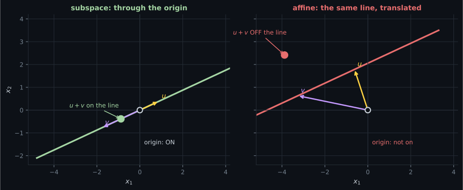
Reading the plot

The second figure is why this section exists at all in a machine learning book.

A hyperplane in $\mathbb{R}^n$ is defined by one linear equation, and one equation removes exactly one dimension — hence $n-1$. That deficiency is not a technicality: it is precisely what allows the object to have two sides. Evaluate $\mathbf{w}^\top\mathbf{x} + b$ at a point and the sign tells you which half-space you are in. A lower-dimensional object, like a line in $\mathbb{R}^3$, does not separate anything — you can walk around it.

So classification by a linear model is: place a hyperplane, and read off signs. The offset $b$ is what lets the hyperplane sit anywhere rather than being forced through the origin — and forcing it through the origin would make a whole class of problems unsolvable, which is the practical reason the bias term exists.

Chapter 12 then asks the natural follow-up: of all the hyperplanes that separate the data, which is best? Its answer is the one furthest from the nearest points, and §3.8’s projections supply the distance.

From the book

Mathematics for Machine Learning §2.8 opens with the remark that “in the machine learning literature, the distinction between linear and affine is sometimes not clear so that we can find references to affine spaces/mappings as linear spaces/mappings”. §2.8.1 gives Definition 2.25 (affine subspace, also linear manifold, Equations 2.130a–b) with $U$ the direction or direction space and $\mathbf{x}_0$ the support point, noting that Chapter 12 refers to such a subspace as a hyperplane. It states explicitly that the definition “excludes $\mathbf{0}$ if $\mathbf{x}_0 \notin U$”, so an affine subspace is not a linear subspace of $V$ in that case, and gives points, lines and planes in $\mathbb{R}^3$ as examples that need not pass through the origin. The containment Remark gives $L \subseteq \tilde{L}$ iff $U \subseteq \tilde{U}$ and $\mathbf{x}_0 - \tilde{\mathbf{x}}_0 \in \tilde{U}$. The parametric equation with directional vectors and parameters is Equation 2.131. Example 2.26 names one-dimensional affine subspaces lines (with Figure 2.13), two-dimensional ones planes, and $(n-1)$-dimensional ones hyperplanes, noting that in $\mathbb{R}^2$ a line is also a hyperplane and in $\mathbb{R}^3$ a plane is also a hyperplane. The Remark on inhomogeneous systems states that the solution of $\mathbf{A}\mathbf{x} = \mathbf{b}$ is either empty or an affine subspace of $\mathbb{R}^n$ of dimension $n - \operatorname{rk}(\mathbf{A})$, that the solution of a single equation $\lambda_1x_1 + \cdots + \lambda_nx_n = b$ with not all $\lambda_i$ zero is a hyperplane, that every $k$-dimensional affine subspace of $\mathbb{R}^n$ is the solution of an inhomogeneous system with $\operatorname{rk}(\mathbf{A}) = n - k$, and that a homogeneous system’s solution subspace can be thought of as a special affine space with support point $\mathbf{x}_0 = \mathbf{0}$. §2.8.2 gives Definition 2.26 (affine mapping, Equations 2.132–2.133) with $\mathbf{a}$ the translation vector, and the three properties: every affine mapping is a uniquely determined composition $\phi = \tau \circ \Phi$ of a linear mapping and a translation, the composition of affine mappings is affine, and affine mappings keep the geometric structure invariant while preserving dimension and parallelism.

Pitfalls

An affine subspace is not a subspace

It fails on two counts when $\mathbf{x}_0 \notin U$: it does not contain $\mathbf{0}$, and it is not closed under addition or scaling. Both were checked numerically above. Calling it a “subspace” because it looks flat is the commonest slip here.

“Hyperplane” has no fixed dimension

It means “one dimension less than the ambient space”. A line in $\mathbb{R}^2$, a plane in $\mathbb{R}^3$, a 999-dimensional object in $\mathbb{R}^{1000}$. When a paper says “separating hyperplane” the dimension is whatever the feature count minus one happens to be.

The support point is not canonical

Any point of the affine subspace works. Two people describing the same plane with different support points and different bases have written the same set. The containment test — directions nest and the offset is a direction — is the way to compare them.

A “linear layer” is affine

$\mathbf{W}\mathbf{x} + \mathbf{b}$ sends $\mathbf{0}$ to $\mathbf{b}$, so it is not linear by §2.7’s definition. The book warns that the literature blurs this. It matters when you reason about composition: a stack of affine maps with no nonlinearity between them collapses to a single affine map, which is why activation functions are not optional.

The augmentation trick costs a dimension

Appending a $1$ turns an affine map in $\mathbb{R}^n$ into a linear map in $\mathbb{R}^{n+1}$, and that is genuinely useful — it is why design matrices have a column of ones. But the augmented vectors live in a bigger space, and the image of the augmented map is an affine subspace of it, not a subspace.

Compare

	subspace	affine subspace
contains $\mathbf{0}$	yes, required	only if $\mathbf{x}_0 \in U$
closed under addition	yes	no
closed under scaling	yes	no
description	$\operatorname{span}[\mathbf{b}_1,\dots,\mathbf{b}_k]$	$\mathbf{x}_0 + \operatorname{span}[\mathbf{b}_1,\dots,\mathbf{b}_k]$
as a solution set	homogeneous $\mathbf{A}\mathbf{x} = \mathbf{0}$	inhomogeneous $\mathbf{A}\mathbf{x} = \mathbf{b}$
the associated mapping	linear, $\Phi(\mathbf{x})$	affine, $\mathbf{a} + \Phi(\mathbf{x})$
in deep learning	$\mathbf{W}\mathbf{x}$	$\mathbf{W}\mathbf{x} + \mathbf{b}$ — what layers actually compute

pch.quizTag Check yourself

1. An affine subspace with support point outside its direction space fails how many of the three subspace conditions?

   A One — it does not contain the zero vector B All three — no zero vector, and closed under neither addition nor scaling C Two — closure under addition and scaling, but it does contain zero D None — it is a subspace
   pch.quizShowAnswer

   B — All three — no zero vector, and closed under neither addition nor scaling — All three. The numerical check on this page shows the sum of two points on the line is off it, and twice a point is off it, in addition to the origin not being on it.

2. What is a hyperplane in R to the 1000?

   A A plane, so two-dimensional B A 999-dimensional affine subspace — always one dimension less than the ambient space C A line D The whole space minus the origin
   pch.quizShowAnswer

   B — A 999-dimensional affine subspace — always one dimension less than the ambient space — Hyperplane means codimension one. One linear equation removes exactly one dimension, and that deficiency is what gives the object two sides — which is what makes it a decision boundary.

3. A neural network layer computes W x plus b. Is it linear?

   A Yes, that is why it is called a linear layer B No — it is affine, because it sends the zero vector to b rather than to zero C Only if b is learned rather than fixed D Only in one dimension
   pch.quizShowAnswer

   B — No — it is affine, because it sends the zero vector to b rather than to zero — The bias is a translation vector, so the map is affine. The book explicitly notes the literature blurs this. It matters because a stack of affine maps with nothing between them collapses to one affine map.

4. Why does appending a constant one to the input turn an affine map into a linear one?

   A It does not — the map is still affine B Because the translation can be absorbed as an extra column, and the augmented input is never the zero vector so the zero test is not violated C Because adding a dimension always linearises a map D Because the constant cancels in the product
   pch.quizShowAnswer

   B — Because the translation can be absorbed as an extra column, and the augmented input is never the zero vector so the zero test is not violated — The bias becomes an extra matrix column acting on the constant one. The augmented map is genuinely linear in the larger space, and the reason no contradiction arises is that the augmented input can never be zero. This is why design matrices carry a column of ones.

🧪 Try It Yourself

Exercise 1 – Is the origin on the line?

pch.exerciseTag pch.exerciseTitle

Exercise 2 – Closure fails

pch.exerciseTag pch.exerciseTitle

Exercise 3 – An inhomogeneous system is a hyperplane

pch.exerciseTag pch.exerciseTitle

Exercise 4 – An affine map is not linear

pch.exerciseTag pch.exerciseTitle

Exercise 5 – The augmentation trick

pch.exerciseTag pch.exerciseTitle

Recall card

• An affine subspace is a subspace slid off the origin — support point plus direction space — and it is not a subspace whenever the support point lies outside the direction space.
• It fails all three subspace conditions: no zero vector, and closure under neither addition nor scaling.
• The support point is not canonical. Any point of the set works, so two different descriptions can name the same set.
• The containment test needs two conditions — the direction spaces nest, and the offset between support points is itself a direction.
• The parametric equation gives a unique representation once the support point and an ordered basis of the direction space are fixed.
• A hyperplane is always one dimension short of the ambient space — a line in the plane, a plane in three dimensions — and that codimension of one is what gives it two sides.
• The solution set of an inhomogeneous system is exactly an affine subspace of dimension $n$ minus the rank, and conversely every affine subspace is such a solution set.
• A single linear equation defines a hyperplane, because one equation removes one dimension.
• A subspace is an affine subspace with support point at the origin — the affine notion is the more general one.
• Every affine mapping is a linear mapping followed by a translation, uniquely determined, and affine mappings preserve dimension and parallelism.
• A “linear layer” computing Wx + b is affine, not linear — the bias is the translation vector, and the book notes the literature blurs this.
• Appending a constant one absorbs the translation into the matrix, turning an affine map in $n$ dimensions into a linear map in $n+1$. That is why design matrices have a column of ones.

Next: Chapter 2 gave you vectors, matrices and the maps between them, all without a notion of length or angle. Chapter 3 adds the geometry — Analytic Geometry.