Linear and Quadratic Programming

Page 704 established what convexity buys. This page spends it. Two families cover an enormous fraction of what actually gets solved:

• Linear programs — linear objective, linear constraints. The book calls them “one of the most widely used approaches in industry”.
• Quadratic programs — convex quadratic objective, linear constraints. Chapter 12’s support vector machine is one.

Both are convex, so strong duality holds and the dual is worth deriving. The derivations follow the same three steps each time, and the single place they diverge explains why their duals look so different.

What you’ll learn

• Equation 7.39 (the LP) and Equation 7.45 (the QP), and what makes each convex.
• The three-step recipe for a Lagrangian dual: write it, collect the terms in $\mathbf{x}$, set the derivative in $\mathbf{x}$ to zero.
• Why that third step produces a constraint for the LP (Equation 7.42) and a substitution for the QP (Equation 7.50) — the whole reason Equations 7.43 and 7.52 have different shapes.
• Example 7.5 solved exactly: $\mathbf{x}^\star = (37/3, 25/6)$, objective $-445/6 = -74.166667$, and $\boldsymbol\lambda^\star = (13/6, 1/3, 0, 0, 0)$.
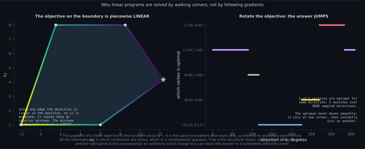
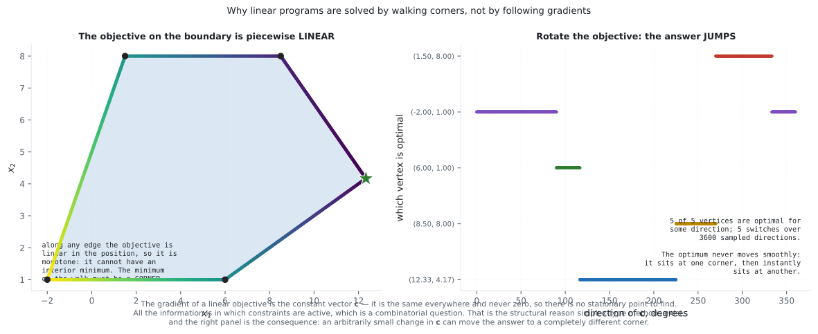
• Why an LP optimum is always a vertex, and the consequence: rotating the objective makes the answer jump. Measured — all $5$ vertices are optimal for some direction, with $5$ switches over $3600$ sampled directions.
• Equation 7.51 checked against a direct evaluation of the Lagrangian: agreement to $1.8\times10^{-14}$ over $20{,}000$ random $\boldsymbol\lambda$.
• How to decide whether to solve the primal or the dual, from $m$ against $d$.

Intuition: a slab, and a bowl in a box

A linear program is a flat sheet tilted over a polygon. There is no bottom of a bowl — the sheet just tilts — so the lowest point is wherever the polygon’s edge stops you. That is always a corner, and you can find it by checking every corner. There is no gradient information to follow, because the gradient of a linear function is the same vector everywhere.

A quadratic program is a bowl in a box. If the bowl’s bottom is inside the box you are done, and the constraints were irrelevant. If it is outside, the answer is pressed against a wall, and the wall pushes back with exactly enough force to hold it — which is the $\lambda^\star = 2.5$ of page 703.

diagram One recipe, and the step where the two families part ways mermaid

  flowchart TD
  S1["step 1: write the Lagrangian
L = f + lambda-transpose (Ax - b)"]
  S1 --> S2["step 2: collect the terms in x"]
  S2 --> LP["LP: L = (c + A-transpose lambda)-transpose x - lambda-transpose b
x appears LINEARLY"]
  S2 --> QP["QP: L = half x-transpose Q x + (c + A-transpose lambda)-transpose x - lambda-transpose b
x appears QUADRATICALLY"]
  LP --> LP3["step 3: d/dx has no x in it,
so Eq 7.42 is a CONSTRAINT on lambda"]
  QP --> QP3["step 3: d/dx can be solved for x,
so Eq 7.50 SUBSTITUTES back"]
  LP3 --> LPD["Eq 7.43: the dual is another LP
m variables, d equality constraints"]
  QP3 --> QPD["Eq 7.52: the dual is a concave quadratic
m variables, lambda >= 0 only"]
  LPD --> Z["both gaps are zero:
convex, so strong duality"]
  QPD --> Z

§7.3.1 Linear Programming

The problem

$$\min_{\mathbf{x}\in\mathbb{R}^d} \mathbf{c}^\top\mathbf{x} \qquad\text{subject to}\qquad \mathbf{A}\mathbf{x} \leq \mathbf{b}$$

with $\mathbf{A} \in \mathbb{R}^{m\times d}$ and $\mathbf{b} \in \mathbb{R}^m$: $d$ variables and $m$ linear constraints. Every $g_i$ is affine and therefore convex, and a linear objective is convex too (its Hessian is the zero matrix, which is positive semidefinite), so this is a convex problem by Equation 7.38.

The dual, in three steps

Step 1. The Lagrangian, with $\boldsymbol\lambda \in \mathbb{R}^m$, $\boldsymbol\lambda \geq 0$:

$$L(\mathbf{x}, \boldsymbol\lambda) = \mathbf{c}^\top\mathbf{x} + \boldsymbol\lambda^\top(\mathbf{A}\mathbf{x} - \mathbf{b})$$

Step 2. Collect the terms containing $\mathbf{x}$:

$$L(\mathbf{x}, \boldsymbol\lambda) = (\mathbf{c} + \mathbf{A}^\top\boldsymbol\lambda)^\top\mathbf{x} - \boldsymbol\lambda^\top\mathbf{b}$$

Step 3. Differentiate in $\mathbf{x}$ and set to zero:

$$\mathbf{c} + \mathbf{A}^\top\boldsymbol\lambda = \mathbf{0}$$

Here is the crucial observation. That equation contains no $\mathbf{x}$. You cannot solve it for $\mathbf{x}$ and substitute back — there is nothing to substitute. Instead read it as a condition on $\boldsymbol\lambda$: unless $\mathbf{c} + \mathbf{A}^\top\boldsymbol\lambda = \mathbf{0}$, the Lagrangian is a nonconstant linear function of $\mathbf{x}$ and its minimum over $\mathbb{R}^d$ is $-\infty$. So $D(\boldsymbol\lambda) = -\boldsymbol\lambda^\top\mathbf{b}$ wherever the dual is finite, and the dual problem is

$$\max_{\boldsymbol\lambda\in\mathbb{R}^m} -\mathbf{b}^\top\boldsymbol\lambda \qquad\text{subject to}\qquad \mathbf{c} + \mathbf{A}^\top\boldsymbol\lambda = \mathbf{0}, \quad \boldsymbol\lambda \geq 0$$

This is another linear program — but with $m$ variables and $d$ equality constraints, exactly the transpose of the primal’s shape. The book’s practical note: choose whichever is smaller. Recall $d$ is the number of variables and $m$ the number of constraints.

Convention

It is convention to minimise the primal and maximise the dual. That is why the primal reads $\min \mathbf{c}^\top\mathbf{x}$ and the dual reads $\max -\mathbf{b}^\top\boldsymbol\lambda$ rather than $\min \mathbf{b}^\top\boldsymbol\lambda$. The two are the same problem; only the sign of the reported value differs.

§7.3.2 Quadratic Programming

The problem

$$\min_{\mathbf{x}\in\mathbb{R}^d} \frac{1}{2}\mathbf{x}^\top\mathbf{Q}\mathbf{x} + \mathbf{c}^\top\mathbf{x} \qquad\text{subject to}\qquad \mathbf{A}\mathbf{x} \leq \mathbf{b}$$

with $\mathbf{Q} \in \mathbb{R}^{d\times d}$ square, symmetric and positive definite. That last condition is what makes the objective convex — its Hessian is $\mathbf{Q}$ itself — and it is also what makes $\mathbf{Q}^{-1}$ exist, which the derivation needs.

The dual, same three steps

Step 1 and 2:

$$L(\mathbf{x}, \boldsymbol\lambda) = \frac{1}{2}\mathbf{x}^\top\mathbf{Q}\mathbf{x} + \mathbf{c}^\top\mathbf{x} + \boldsymbol\lambda^\top(\mathbf{A}\mathbf{x} - \mathbf{b}) = \frac{1}{2}\mathbf{x}^\top\mathbf{Q}\mathbf{x} + (\mathbf{c} + \mathbf{A}^\top\boldsymbol\lambda)^\top\mathbf{x} - \boldsymbol\lambda^\top\mathbf{b}$$

Step 3. Differentiate in $\mathbf{x}$ and set to zero:

$$\mathbf{Q}\mathbf{x} + (\mathbf{c} + \mathbf{A}^\top\boldsymbol\lambda) = \mathbf{0}$$

Now the $\mathbf{x}$ is there, because the objective was quadratic. Assuming $\mathbf{Q}$ is invertible,

$$\mathbf{x} = -\mathbf{Q}^{-1}(\mathbf{c} + \mathbf{A}^\top\boldsymbol\lambda)$$

so we can substitute back. Writing $\mathbf{v} = \mathbf{c} + \mathbf{A}^\top\boldsymbol\lambda$ and using $\tfrac12\mathbf{v}^\top\mathbf{Q}^{-1}\mathbf{v} - \mathbf{v}^\top\mathbf{Q}^{-1}\mathbf{v} = -\tfrac12\mathbf{v}^\top\mathbf{Q}^{-1}\mathbf{v}$:

$$D(\boldsymbol\lambda) = -\frac{1}{2}(\mathbf{c} + \mathbf{A}^\top\boldsymbol\lambda)^\top\mathbf{Q}^{-1}(\mathbf{c} + \mathbf{A}^\top\boldsymbol\lambda) - \boldsymbol\lambda^\top\mathbf{b}$$

and the dual problem is

$$\max_{\boldsymbol\lambda\in\mathbb{R}^m} -\frac{1}{2}(\mathbf{c} + \mathbf{A}^\top\boldsymbol\lambda)^\top\mathbf{Q}^{-1}(\mathbf{c} + \mathbf{A}^\top\boldsymbol\lambda) - \boldsymbol\lambda^\top\mathbf{b} \qquad\text{subject to}\qquad \boldsymbol\lambda \geq 0$$

A concave quadratic in $\boldsymbol\lambda$ with only the sign constraint — no equalities. Chapter 12 applies exactly this, and the $\mathbf{Q}^{-1}$ becomes the kernel matrix.

Where positive definiteness is load-bearing

The book says $\mathbf{Q}$ is positive definite, and then Equation 7.50 says “assuming that $\mathbf{Q}$ is invertible”. Those are the same assumption stated twice, and both steps need it. If $\mathbf{Q}$ were only positive semidefinite the objective would still be convex, but $\mathbf{Q}^{-1}$ would not exist and Equation 7.50 would have no unique solution — the inner minimisation would have a flat direction. The measured eigenvalues of Example 7.6’s $\mathbf{Q}$ are $1.585786$ and $4.414214$, both strictly positive.

Worked example by hand

Example 7.5, the linear program

$$\min_{\mathbf{x}\in\mathbb{R}^2} -\begin{bmatrix}5\\3\end{bmatrix}^\top\begin{bmatrix}x_1\\x_2\end{bmatrix} \qquad\text{subject to}\qquad \begin{bmatrix}2&2\\2&-4\\-2&1\\0&-1\\0&1\end{bmatrix}\begin{bmatrix}x_1\\x_2\end{bmatrix} \leq \begin{bmatrix}33\\8\\5\\-1\\8\end{bmatrix}$$

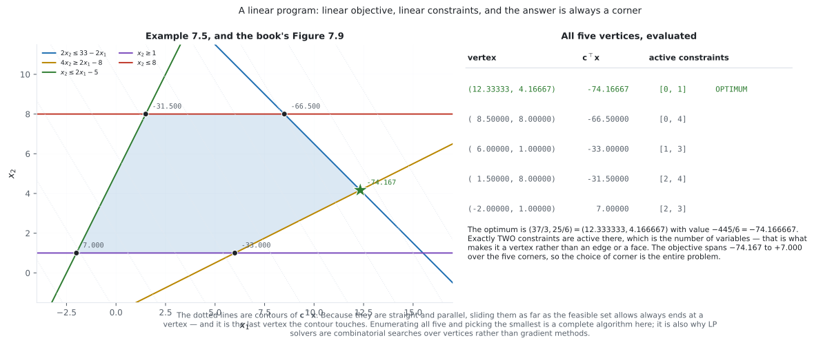
$d = 2$, $m = 5$. Minimising $-5x_1 - 3x_2$ means maximising $5x_1 + 3x_2$, so we are pushing up and to the right — matching the book’s Figure 7.9 caption.

Step 1: find the vertices. A vertex in $\mathbb{R}^2$ is where two constraint boundaries cross, so solve each of the $\binom{5}{2} = 10$ pairs and keep the feasible ones. Five survive:

vertex	$\mathbf{c}^\top\mathbf{x}$	active constraints
$(12.33333,\ 4.16667)$	$\mathbf{-74.16667}$	$0, 1$
$(8.5,\ 8)$	$-66.5$	$0, 4$
$(6,\ 1)$	$-33$	$1, 3$
$(1.5,\ 8)$	$-31.5$	$2, 4$
$(-2,\ 1)$	$+7$	$2, 3$

Step 2: read off the winner. The optimum is the first row. Solving rows $0$ and $1$ exactly:

$$2x_1 + 2x_2 = 33, \qquad 2x_1 - 4x_2 = 8$$

Subtracting gives $6x_2 = 25$, so $x_2 = 25/6$, and then $x_1 = (33 - 25/3)/2 = 37/3$. Check: $2(37/3) + 2(25/6) = 74/3 + 25/3 = 33$ ✓.

$$\mathbf{x}^\star = \left(\frac{37}{3}, \frac{25}{6}\right), \qquad \mathbf{c}^\top\mathbf{x}^\star = -\frac{185}{3} - \frac{25}{2} = -\frac{445}{6} = -74.166667$$

Step 3: the dual. Only the two active constraints can carry a nonzero multiplier (complementary slackness), so solve $\mathbf{A}_{\text{act}}^\top\boldsymbol\lambda_{\text{act}} = -\mathbf{c}$:

$$\begin{bmatrix}2&2\\2&-4\end{bmatrix}^\top\begin{bmatrix}\lambda_0\\\lambda_1\end{bmatrix} = \begin{bmatrix}2&2\\2&-4\end{bmatrix}\begin{bmatrix}\lambda_0\\\lambda_1\end{bmatrix} = \begin{bmatrix}5\\3\end{bmatrix}$$

Subtracting: $6\lambda_1 = 2$, so $\lambda_1 = 1/3$, and $\lambda_0 = (5 - 2/3)/2 = 13/6$. Both positive, as required. So

$$\boldsymbol\lambda^\star = \left(\frac{13}{6}, \frac{1}{3}, 0, 0, 0\right), \qquad -\mathbf{b}^\top\boldsymbol\lambda^\star = -\left(33\cdot\frac{13}{6} + 8\cdot\frac{1}{3}\right) = -\left(\frac{143}{2} + \frac{8}{3}\right) = -\frac{445}{6}$$

The same $-445/6$. Duality gap zero, exactly as strong duality promised.

Example 7.6, the quadratic program

Page 703 solved this one: $\mathbf{x}^\star = (-1, -1/2)$ with $f = -4.5$ and $\boldsymbol\lambda^\star = (0, 2.5, 0, 0)$. What is new here is that Equation 7.51 gives the dual objective in closed form, so it can be maximised directly rather than by solving the primal. With $\det\mathbf{Q} = 7$,

$$\mathbf{Q}^{-1} = \frac{1}{7}\begin{bmatrix}4&-1\\-1&2\end{bmatrix}$$

and at $\boldsymbol\lambda = (0, \lambda, 0, 0)$ we have $\mathbf{v} = \mathbf{c} + \mathbf{A}^\top\boldsymbol\lambda = (5 - \lambda, 3)$, so

$$D(\lambda) = -\frac{1}{14}\Big(4(5-\lambda)^2 - 2(5-\lambda)(3) + 2(9)\Big) - \lambda$$

Expanding: $-\tfrac{1}{14}(4\lambda^2 - 34\lambda + 88) - \lambda = -\tfrac{2}{7}\lambda^2 + \tfrac{17}{7}\lambda - \tfrac{44}{7} - \lambda$. Differentiating and setting to zero: $-\tfrac{4}{7}\lambda + \tfrac{10}{7} = 0$, so $\lambda^\star = 2.5$, and $D(2.5) = -\tfrac{2}{7}(6.25) + \tfrac{10}{7}(2.5) - \tfrac{44}{7} = \tfrac{-12.5 + 25 - 44}{7} = -\tfrac{31.5}{7} = -4.5$ ✓.

See it move

An LP is a combinatorial problem wearing continuous clothes. Rotate the objective and watch:

sketch Rotate the objective and watch the answer jump between corners p5.js Pause Restart

Example 7.5's feasible pentagon with a rotating objective direction. The optimal vertex is starred and the objective contour is drawn through it. Nothing moves continuously: the answer sits at one corner until a threshold, then instantly sits at another.

From scratch

lp_and_qp.py

import itertools
 
import numpy as np
 
# ---- Example 7.5, Equation 7.44 ------------------------------------------
c = np.array([-5.0, -3.0])
A = np.array([[2.0, 2.0], [2.0, -4.0], [-2.0, 1.0],
              [0.0, -1.0], [0.0, 1.0]])
b = np.array([33.0, 8.0, 5.0, -1.0, 8.0])
 
def feasible(x):
    return bool(np.all(A @ x <= b + 1e-9))
 
# An LP optimum is at a vertex, and a vertex is where two constraints meet.
# With only five constraints we can just enumerate all of them.
verts = []
for i, j in itertools.combinations(range(len(b)), 2):
    M = A[[i, j]]
    if abs(np.linalg.det(M)) < 1e-12:
        continue                       # parallel boundaries never meet
    v = np.linalg.solve(M, b[[i, j]])
    if feasible(v) and not any(np.allclose(v, w, atol=1e-9) for w in verts):
        verts.append(v)
verts = np.array(verts)
 
print(f"{len(verts)} feasible vertices, sorted by objective:")
for v in verts[np.argsort(verts @ c)]:
    act = [i for i, q in enumerate(A @ v - b) if abs(q) < 1e-9]
    print(f"  [{v[0]:9.5f}, {v[1]:9.5f}]   c^T x = {v @ c:10.5f}   "
          f"active {act}")
xstar = verts[int(np.argmin(verts @ c))]
print(f"\nx* = ({xstar[0]:.6f}, {xstar[1]:.6f}) = (37/3, 25/6)")
print(f"c^T x* = {xstar @ c:.6f} = -445/6")
 
# ---- Equation 7.43, the dual LP -----------------------------------------
# max -b^T lam  s.t.  c + A^T lam = 0,  lam >= 0.
# Only the two active constraints can carry a nonzero multiplier, so solve
# the 2x2 system on those and check the rest are zero.
act = [i for i, q in enumerate(A @ xstar - b) if abs(q) < 1e-9]
lam = np.zeros(len(b))
lam[act] = np.linalg.solve(A[act].T, -c)
print(f"\nlambda* = {np.round(lam, 6).tolist()}")
print(f"  as fractions: 13/6 = {13/6:.6f}, 1/3 = {1/3:.6f}")
print(f"  stationarity c + A^T lambda = {np.round(c + A.T @ lam, 9).tolist()}")
print(f"  all multipliers non-negative: {bool(np.all(lam >= -1e-12))}")
print(f"  dual objective -b^T lambda = {-(b @ lam):.6f}")
print(f"  primal objective c^T x*    = {xstar @ c:.6f}")
print(f"  duality gap = {abs(xstar @ c - (-(b @ lam))):.3e}")
print(f"\n  primal: {A.shape[1]} variables, {A.shape[0]} constraints")
print(f"  dual  : {A.shape[0]} variables, {A.shape[1]} equality constraints")
 
# ---- the optimum is a corner, and it JUMPS ------------------------------
print("\nRotating the objective direction through 360 degrees:")
angles = np.linspace(0, 2 * np.pi, 3601)
winners = np.array([int(np.argmin(verts @ np.array([np.cos(a), np.sin(a)])))
                    for a in angles])
print(f"  distinct vertices that are ever optimal: "
      f"{len(set(winners.tolist()))} of {len(verts)}")
print(f"  switches over 3600 sampled directions : "
      f"{int((np.diff(winners) != 0).sum())}")
for k, v in enumerate(verts):
    print(f"    ({v[0]:8.4f}, {v[1]:7.4f}) is optimal over "
          f"{360 * (winners == k).mean():5.1f} degrees")
 
# ---- Example 7.6, the QP, and Equation 7.51 ----------------------------
print("\n--- the quadratic program ---------------------------------------")
Q = np.array([[2.0, 1.0], [1.0, 4.0]])
cq = np.array([5.0, 3.0])
Aq = np.array([[1.0, 0.0], [-1.0, 0.0], [0.0, 1.0], [0.0, -1.0]])
bq = np.ones(4)
Qinv = np.linalg.inv(Q)
 
print(f"Q eigenvalues {np.linalg.eigvalsh(Q).round(6).tolist()} -> "
      f"positive definite, so Q^-1 exists")
 
def primal(x):
    return 0.5 * x @ Q @ x + cq @ x
 
def x_of_lam(l):
    """Equation 7.50."""
    return -Qinv @ (cq + Aq.T @ l)
 
def dual(l):
    """Equation 7.51."""
    v = cq + Aq.T @ l
    return -0.5 * v @ Qinv @ v - l @ bq
 
# Equation 7.51 must equal the Lagrangian evaluated at Equation 7.50.
rng = np.random.default_rng(0)
worst = 0.0
for _ in range(20000):
    l = rng.uniform(0, 4, 4)
    x = x_of_lam(l)
    worst = max(worst, abs((primal(x) + l @ (Aq @ x - bq)) - dual(l)))
print(f"max |L(x(lambda), lambda) - D(lambda)| over 20000 draws: {worst:.3e}")
 
ts = np.linspace(0.0, 6.0, 60001)
dv = np.array([dual(np.array([0.0, t, 0.0, 0.0])) for t in ts])
k = int(np.argmax(dv))
lam_q = np.array([0.0, ts[k], 0.0, 0.0])
xq = np.array([-1.0, -0.5])
print(f"\nlambda* = {np.round(lam_q, 6).tolist()}")
print(f"d* = {dual(lam_q):.9f}   p* = {primal(xq):.9f}   "
      f"gap = {abs(primal(xq) - dual(lam_q)):.3e}")
print(f"x from Eq 7.50 = {np.round(x_of_lam(lam_q), 6).tolist()}   "
      f"matches x*: {np.allclose(x_of_lam(lam_q), xq, atol=1e-6)}")

text

5 feasible vertices, sorted by objective:
  [ 12.33333,   4.16667]   c^T x =  -74.16667   active [0, 1]
  [  8.50000,   8.00000]   c^T x =  -66.50000   active [0, 4]
  [  6.00000,   1.00000]   c^T x =  -33.00000   active [1, 3]
  [  1.50000,   8.00000]   c^T x =  -31.50000   active [2, 4]
  [ -2.00000,   1.00000]   c^T x =    7.00000   active [2, 3]
 
x* = (12.333333, 4.166667) = (37/3, 25/6)
c^T x* = -74.166667 = -445/6
 
lambda* = [2.166667, 0.333333, 0.0, 0.0, 0.0]
  as fractions: 13/6 = 2.166667, 1/3 = 0.333333
  stationarity c + A^T lambda = [0.0, 0.0]
  all multipliers non-negative: True
  dual objective -b^T lambda = -74.166667
  primal objective c^T x*    = -74.166667
  duality gap = 1.421e-14
 
  primal: 2 variables, 5 constraints
  dual  : 5 variables, 2 equality constraints
 
Rotating the objective direction through 360 degrees:
  distinct vertices that are ever optimal: 5 of 5
  switches over 3600 sampled directions : 5
    ( 12.3333,  4.1667) is optimal over 108.5 degrees
    (  8.5000,  8.0000) is optimal over  45.0 degrees
    (  6.0000,  1.0000) is optimal over  26.5 degrees
    ( -2.0000,  1.0000) is optimal over 116.7 degrees
    (  1.5000,  8.0000) is optimal over  63.4 degrees
 
--- the quadratic program ---------------------------------------
Q eigenvalues [1.585786, 4.414214] -> positive definite, so Q^-1 exists
max |L(x(lambda), lambda) - D(lambda)| over 20000 draws: 1.776e-14
 
lambda* = [0.0, 2.5, 0.0, 0.0]
d* = -4.500000000   p* = -4.500000000   gap = 0.000e+00
x from Eq 7.50 = [-1.0, -0.5]   matches x*: True

On real data

figure Example 7.5, and the book's Figure 7.9 matplotlib

Five feasible vertices, objective values spanning minus 74.167 to plus 7. The optimum is at 37 over 3 comma 25 over 6 with value minus 445 over 6, where exactly two constraints are active — matching the two variables.

figure Why linear programs are solved by walking corners matplotlib

The objective is linear along each edge, so it is monotone and cannot have an interior minimum — the answer must be a corner. Rotating the objective, all five vertices win for some direction, with five switches over 3600 sampled directions.

figure Two convex families, two duals, and both gaps are zero matplotlib

The linear program's dual is another linear program with the roles of variables and constraints swapped. The quadratic program's dual is a concave quadratic, and Equation 7.51 reproduces a direct evaluation of the Lagrangian to 1.8e-14 over 20000 random multipliers.

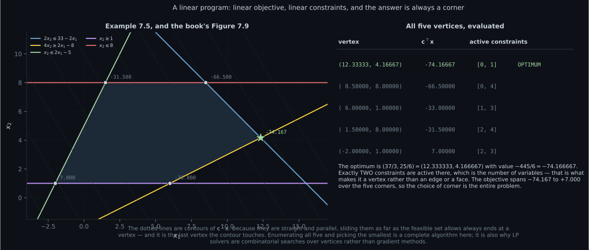
Reading the plot

The first figure removes all the guesswork from Example 7.5. The five coloured lines are the constraint boundaries, the shaded pentagon is where all five hold, and the dotted lines are contours of $\mathbf{c}^\top\mathbf{x}$ — straight and parallel, because the objective is linear. The table on the right evaluates every vertex, and the point of listing all five is that the objective ranges from $-74.167$ to $+7$ across them. Picking the right corner is the entire problem; there is no gradient step that gets you there.

The active-constraint column is worth reading closely. Every vertex has exactly two active constraints, and there are exactly two variables. That is not a coincidence: a point in $\mathbb{R}^d$ is pinned by $d$ independent equalities, so a vertex needs $d$ active constraints. Fewer and you are on an edge or a face and can still move; more and the constraints are degenerate. This is the fact that turns an LP into a finite search: there are at most $\binom{m}{d}$ candidate vertices, here $\binom{5}{2} = 10$, of which five turned out feasible.

The second figure explains why no amount of calculus helps. The left panel colours the boundary by objective value, and along each edge the colour changes linearly — because $\mathbf{c}^\top\mathbf{x}$ restricted to a line segment is an affine function of position. An affine function on an interval is monotone, so its minimum is at an endpoint. Walk the whole boundary and every local minimum is a corner. There is nowhere else for the answer to be.

Say the same thing with derivatives: $\nabla(\mathbf{c}^\top\mathbf{x}) = \mathbf{c}$, a constant nonzero vector. There is no stationary point anywhere. Everything page 701 built assumed you were looking for a place where the gradient vanishes, and here no such place exists. All the information lives in which constraints are active, which is a discrete question — and that is the structural reason simplex-type methods walk from vertex to vertex instead of following a slope.

The right panel shows the price of that discreteness. Sweeping the objective direction through $360°$, all five vertices are optimal for some range of directions, and there are exactly five switches. Each vertex owns a contiguous arc — $108.5°$ for the winner at $(12.33, 4.17)$, only $26.5°$ for $(6, 1)$ — and the arcs sum to $360°$. Between arcs the answer does not drift; it teleports. So an arbitrarily small change in $\mathbf{c}$ can move the solution to a completely different point, which matters whenever $\mathbf{c}$ comes from estimated data.

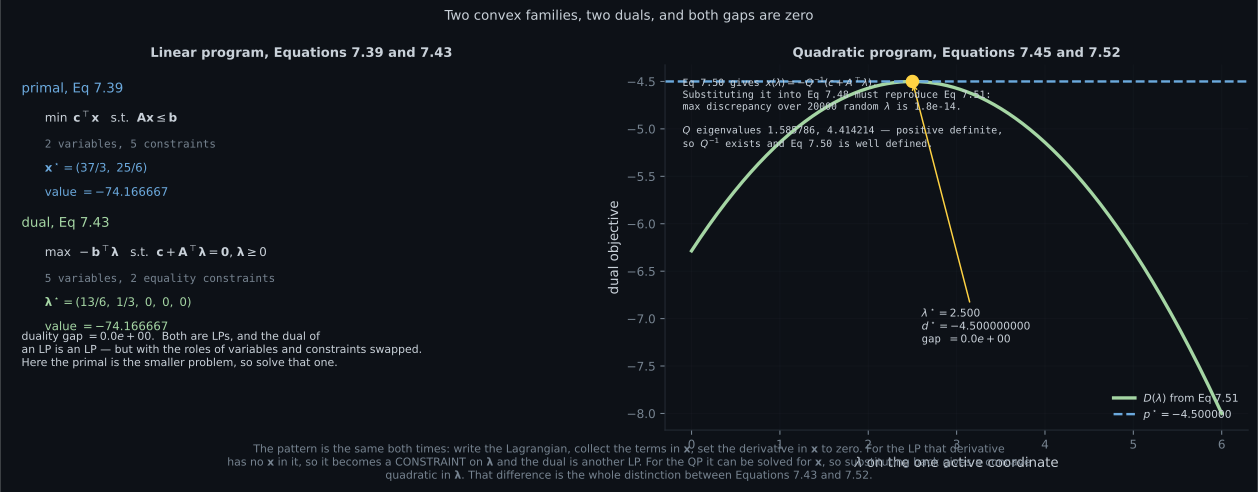
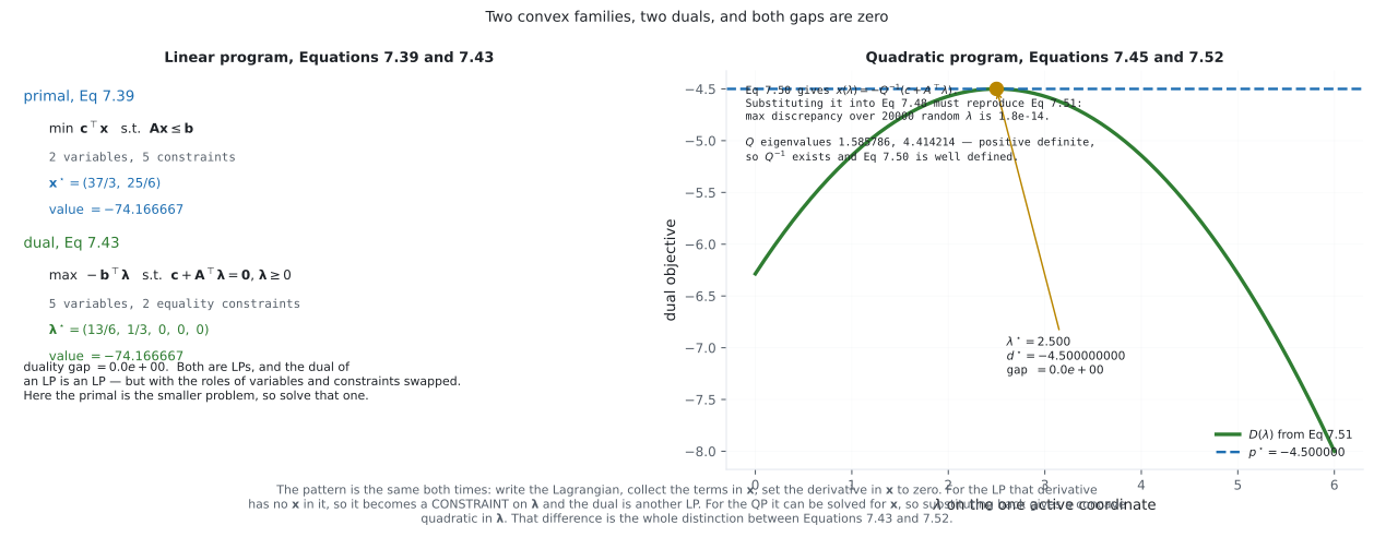
The third figure is the payoff of the three-step recipe. The left panel puts the LP’s primal and dual side by side, and the shapes are transposed: $2$ variables with $5$ constraints becomes $5$ variables with $2$ equality constraints. Both reach $-74.166667$, gap $1.4\times10^{-14}$. For this problem the primal is the smaller one, so the book’s advice — solve whichever is smaller — says solve the primal. The advice earns its keep in the other direction: an SVM with $10^6$ training points and $10$ features has a dual with $10^6$ variables and a primal with $10$, and Chapter 12 nonetheless solves the dual, because the dual is where the kernel trick lives. “Smaller” is a heuristic, not a rule.

The right panel is Equation 7.51 doing real work. It is a closed-form dual objective — no inner minimisation left to perform — and the curve is a concave parabola in $\lambda$ whose peak sits exactly on $p^\star = -4.5$. The verification in the corner is the one I would not have wanted to skip: substituting Equation 7.50 back into the Lagrangian must reproduce Equation 7.51 algebraically, and over $20{,}000$ random $\boldsymbol\lambda$ the largest discrepancy was $1.776\times10^{-14}$ — floating-point noise. The derivation is right.

From the book

This page covers §7.3.1 and §7.3.2 of Mathematics for Machine Learning by Deisenroth, Faisal and Ong (draft of 2019-12-11). Equation 7.39 is the linear program, 7.40 its Lagrangian, 7.41 the collected form, 7.42 the stationarity condition, and 7.43 the dual linear program. Example 7.5 and Figure 7.9 are the two-variable LP with five constraints. Equation 7.45 is the quadratic program with $\mathbf{Q}$ positive definite, 7.48a and 7.48b its Lagrangian, 7.49 the stationarity condition, 7.50 the solution for $\mathbf{x}$, 7.51 the dual Lagrangian, and 7.52 the dual quadratic program. Example 7.6 and Figure 7.4 are the box-constrained QP. The remark that linear programs “are one of the most widely used approaches in industry”, the note that it is convention to minimise the primal and maximise the dual, and the pointer to Chapter 12 for an application of quadratic programming are all the book’s. The exact vertex enumeration, the fractions $37/3$, $25/6$, $-445/6$, $13/6$ and $1/3$, the rotating-objective measurement, and the numerical verification of Equation 7.51 are this module’s additions.

Pitfalls

Looking for a stationary point of a linear program

$\nabla(\mathbf{c}^\top\mathbf{x}) = \mathbf{c}$, which is constant and nonzero. There is no stationary point. Any solver or convergence test built around $\lVert\nabla f\rVert \to 0$ will never terminate on an LP. The optimum is characterised by which constraints are active, not by a vanishing derivative.

Expecting the LP solution to move smoothly with the data

Measured on Example 7.5: sweeping the objective direction through $360°$ produces five abrupt switches and no continuous motion. Each vertex owns an arc — the narrowest is $26.5°$ — and at the boundary between arcs the answer jumps to a different point entirely. If $\mathbf{c}$ is estimated from noisy data, a small perturbation can change the answer completely, and reporting the solution without that sensitivity is misleading.

Applying Equation 7.50 when Q is only semidefinite

Equation 7.50 requires $\mathbf{Q}^{-1}$. A positive semidefinite $\mathbf{Q}$ still gives a convex objective, so the problem is perfectly well posed — but $\mathbf{Q}$ is singular, the inner minimisation has a flat direction, and the substitution into Equation 7.51 is invalid. Example 7.6’s eigenvalues are $1.585786$ and $4.414214$, both strictly positive, which is what licenses the derivation. Check the eigenvalues before using the closed form.

Choosing the primal or dual on size alone

The book’s rule of thumb — solve whichever of $m$ and $d$ is smaller — is a good default and not the whole story. Example 7.5’s primal is smaller ($2$ variables against $5$). But Chapter 12 solves the SVM dual even when it has vastly more variables, because the dual is where the objective depends on the data only through inner products. Structure can outweigh size.

Assuming every vertex is a candidate worth checking

There are $\binom{m}{d}$ intersections of constraint boundaries — here $\binom{5}{2} = 10$ — and only five of them were feasible. The other five satisfy their own two constraints and violate a third. Enumeration must test feasibility against all constraints, not just the two that defined the point.

Reading a zero multiplier as an unimportant constraint

$\boldsymbol\lambda^\star = (13/6, 1/3, 0, 0, 0)$ says three constraints have zero price at this optimum. Rotate the objective and different constraints become active, and their multipliers become nonzero. A zero multiplier means “not binding here”, not “removable from the problem”.

Compare

	linear program, Eq 7.39	quadratic program, Eq 7.45
objective	$\mathbf{c}^\top\mathbf{x}$	$\tfrac12\mathbf{x}^\top\mathbf{Q}\mathbf{x} + \mathbf{c}^\top\mathbf{x}$
Hessian	$\mathbf{0}$	$\mathbf{Q}$, positive definite
contours	parallel straight lines	concentric ellipses
stationary point of the objective	none	exactly one, at $-\mathbf{Q}^{-1}\mathbf{c}$
where the optimum lives	always a vertex	vertex, edge, or interior
step 3 of the dual recipe	Eq 7.42, a constraint on $\boldsymbol\lambda$	Eq 7.50, a substitution for $\mathbf{x}$
the dual	another LP, Eq 7.43	concave quadratic, Eq 7.52
dual constraints	$\mathbf{c} + \mathbf{A}^\top\boldsymbol\lambda = \mathbf{0}$ and $\boldsymbol\lambda \geq 0$	$\boldsymbol\lambda \geq 0$ only
measured gap	$1.4\times10^{-14}$	$0.0$
shows up in	resource allocation, transport, $\ell_1$ problems	SVM (Ch 12), portfolio choice, MPC

pch.quizTag Do you know why these two families behave differently?

1. Why is the optimum of a linear program always at a vertex?

   A Because the feasible set is a polygon and polygons have vertices B Because the objective restricted to any edge is affine in position, hence monotone, so it has no interior minimum C Because the gradient vanishes only at vertices D Because the constraints are linear
   pch.quizShowAnswer

   B — Because the objective restricted to any edge is affine in position, hence monotone, so it has no interior minimum — An affine function on an interval attains its minimum at an endpoint. Walk the boundary and every local minimum is a corner. Saying it with derivatives: the gradient of c-transpose x is the constant vector c, so there is no stationary point anywhere — the whole answer is in which constraints are active, which is a discrete question.

2. In deriving the dual, step 3 sets the derivative in x to zero. What is different between the LP and the QP there?

   A Nothing; both give a formula for x B For the LP that equation contains no x, so it becomes a constraint on lambda; for the QP it can be solved for x and substituted back C The LP requires the constraint gradients while the QP does not D The QP needs the constraints to be equalities
   pch.quizShowAnswer

   B — For the LP that equation contains no x, so it becomes a constraint on lambda; for the QP it can be solved for x and substituted back — c + A-transpose lambda = 0 has no x in it, so there is nothing to substitute — it becomes Equation 7.43's equality constraint, and the dual is another LP. Qx + (c + A-transpose lambda) = 0 does contain x, so Equation 7.50 solves for it and substituting gives the concave quadratic of Equation 7.51. That single step is the entire difference.

3. Example 7.5 has 2 variables and 5 constraints. How many constraints are active at each vertex?

   A All five, since the point must satisfy all of them B Exactly two, matching the number of variables C It varies between one and five D At least three, since a vertex is a corner of a pentagon
   pch.quizShowAnswer

   B — Exactly two, matching the number of variables — A point in d dimensions is pinned by d independent equalities. Fewer active constraints and you are on an edge with room to move; more and the constraints are degenerate. Measured, all five vertices had exactly two active — which is what bounds the search to at most 5-choose-2 = 10 candidates.

4. What does rotating an LP's objective direction do to the optimal point?

   A Moves it smoothly around the boundary of the feasible set B Makes it jump between vertices: measured, all 5 vertices win over contiguous arcs with 5 abrupt switches in 360 degrees C Leaves it fixed as long as the feasible set does not change D Moves it into the interior for some directions
   pch.quizShowAnswer

   B — Makes it jump between vertices: measured, all 5 vertices win over contiguous arcs with 5 abrupt switches in 360 degrees — Each vertex is optimal over a contiguous arc of directions — from 26.5 degrees for one to 108.5 for another, summing to 360 — and at an arc boundary the answer teleports. So a small change in an estimated c can move the solution to a completely different point, which is a real risk when c comes from data.

5. Equation 7.50 writes x = -Q inverse times (c + A-transpose lambda). When is that step invalid?

   A Whenever there are inequality constraints B When Q is positive semidefinite but singular: the objective is still convex, but Q inverse does not exist and the inner minimisation has a flat direction C When lambda has any zero entries D When A is not square
   pch.quizShowAnswer

   B — When Q is positive semidefinite but singular: the objective is still convex, but Q inverse does not exist and the inner minimisation has a flat direction — Convexity only needs Q positive semidefinite; the closed-form dual needs it strictly positive definite. Example 7.6's eigenvalues are 1.585786 and 4.414214, both positive, which is what licenses the derivation — so check the eigenvalues before reaching for Equation 7.51.

🧪 Try It Yourself

Exercise 1 – Enumerate the vertices

pch.exerciseTag pch.exerciseTitle

Exercise 2 – A vertex has as many active constraints as variables

pch.exerciseTag pch.exerciseTitle

Exercise 3 – The dual linear program

pch.exerciseTag pch.exerciseTitle

Exercise 4 – Rotate the objective and the answer jumps

pch.exerciseTag pch.exerciseTitle

Exercise 5 – Equation 7.51 is Equation 7.50 substituted back

pch.exerciseTag pch.exerciseTitle

Recall card

• A linear program, Eq 7.39: minimise c-transpose x subject to Ax at most b. d variables, m constraints. Convex, because a linear objective has a zero Hessian and affine constraints are convex.
• A quadratic program, Eq 7.45: minimise half x-transpose Q x plus c-transpose x subject to Ax at most b, with Q symmetric POSITIVE DEFINITE. That is what makes the objective convex and Q invertible.
• One recipe, three steps: write the Lagrangian, collect the terms in x, set the derivative in x to zero. Both duals come out of the same procedure.
• The two families part at step 3. For the LP, c + A-transpose lambda = 0 contains no x, so it becomes a CONSTRAINT on lambda and the dual is another LP (Eq 7.43). For the QP, Qx + (c + A-transpose lambda) = 0 does contain x, so Eq 7.50 solves for it and substituting gives a concave quadratic (Eq 7.51 and 7.52).
• The LP dual has the transposed shape: m variables and d equality constraints. The book’s advice is to solve whichever of m and d is smaller — a default, not a rule, since Chapter 12 solves the larger SVM dual for structural reasons.
• An LP optimum is always a vertex, because the objective along any edge is affine and therefore monotone. Equivalently: the gradient of a linear objective is the constant vector c, so there is NO stationary point and no gradient method applies.
• A vertex in d dimensions has exactly d active constraints. Measured on Example 7.5: all five vertices had exactly two, with two variables. That bounds the search to at most m-choose-d candidates.
• Example 7.5 exactly: five feasible vertices out of ten intersections, objective from -74.167 to +7. x-star = (37/3, 25/6), value -445/6 = -74.166667, lambda-star = (13/6, 1/3, 0, 0, 0), gap 1.4e-14.
• The LP answer JUMPS. Rotating the objective through 360 degrees: all five vertices win over contiguous arcs (from 26.5 to 116.7 degrees), with exactly five switches. A small change in an estimated c can relocate the solution entirely.
• Eq 7.51 verified: substituting Eq 7.50 into the Lagrangian reproduces the closed-form dual to 1.8e-14 over 20000 random multipliers. Example 7.6’s Q eigenvalues are 1.585786 and 4.414214.
• Positive SEMIdefinite is not enough for Eq 7.50. The objective stays convex, but Q is singular, the inner minimisation has a flat direction, and the closed form is invalid. Check eigenvalues first.
• A zero multiplier means “not binding here”, not “removable”. Rotate the objective and different constraints activate, and their prices become nonzero.

Next: duality without constraints, and the transform that turns a function into a function of its own slopes. Legendre-Fenchel Transform and Convex Conjugate