
End-to-End Machine Learning Project (California Housing)
What you’ll learn
Section titled “What you’ll learn”- the complete project as one runnable script, from CSV to a saved model
- how to shortlist models fast, and read the training-versus-CV gap as a diagnosis
- grid search over preprocessing and model hyperparameters together
- error analysis: which features mattered, and where the model is still wrong
- how to open the test set once, and report a confidence interval rather than a point
- what to hand over, and what to monitor afterwards
The whole project
Section titled “The whole project”flowchart TD A["1 Frame the problem
regression, RMSE, beat 15%"] --> B["2 Get the data
20,640 x 10"] B --> C["3 Split first
stratified on income"] C --> D["4 Explore the training copy
map, correlations, ratios"] D --> E["5 Build the pipeline
impute, engineer, encode, scale"] E --> F["6 Shortlist models
cross-validate all of them"] F --> G["7 Tune the winner
grid search"] G --> H["8 Analyse the errors
importances, residuals"] H --> I["9 Evaluate once
test set + confidence interval"] I --> J["10 Ship and monitor"]
Steps 1 to 5 are the previous six pages. This page runs 6 to 10.
Recap: getting to a prepared matrix
Section titled “Recap: getting to a prepared matrix”import numpy as np
import pandas as pd
from sklearn.compose import ColumnTransformer
from sklearn.impute import SimpleImputer
from sklearn.model_selection import StratifiedShuffleSplit
from sklearn.pipeline import Pipeline
from sklearn.preprocessing import OneHotEncoder, StandardScaler
URL = ("https://raw.githubusercontent.com/ageron/handson-ml2/master/"
"datasets/housing/housing.csv")
housing = pd.read_csv(URL)
# --- 3. Split first, stratified on income -------------------------------
housing["income_cat"] = pd.cut(housing["median_income"],
bins=[0.0, 1.5, 3.0, 4.5, 6.0, np.inf],
labels=[1, 2, 3, 4, 5])
splitter = StratifiedShuffleSplit(n_splits=1, test_size=0.2, random_state=42)
train_idx, test_idx = next(splitter.split(housing, housing["income_cat"]))
train = housing.iloc[train_idx].drop(columns=["income_cat"])
test = housing.iloc[test_idx].drop(columns=["income_cat"])
X_train = train.drop(columns=["median_house_value"])
y_train = train["median_house_value"]
X_test = test.drop(columns=["median_house_value"])
y_test = test["median_house_value"]
print(len(X_train), len(X_test)) # 16512 4128
# --- 5. One preprocessing object ----------------------------------------
num_attribs = X_train.select_dtypes("number").columns.tolist()
cat_attribs = ["ocean_proximity"]
num_pipeline = Pipeline([
("imputer", SimpleImputer(strategy="median")),
("scaler", StandardScaler()),
])
preparation = ColumnTransformer([
("num", num_pipeline, num_attribs),
("cat", OneHotEncoder(handle_unknown="ignore"), cat_attribs),
])The test set now sits untouched until the last section of this page.
Why StratifiedShuffleSplit and not train_test_split
Section titled “Why StratifiedShuffleSplit and not train_test_split”The five income categories are not evenly sized — measured over all 20,640 districts they are 3.98%, 31.88%, 35.06%, 17.63% and 11.44%. A plain random 20% test set reproduces those shares only up to sampling noise, and the smallest category is where the noise bites. Averaged over 200 seeds:
| Split | Mean skew across categories | Mean worst category | Worst seen in 200 seeds |
|---|---|---|---|
train_test_split | 2.788% | 6.531% | 22.141% |
StratifiedShuffleSplit | — | 0.365% | 0.365% |
At random_state=42 specifically, the random split is off by 5.06% on category 4 and 4.32% on
category 5, while the stratified split’s largest error is 0.365% — and that residual is only there
because 4,128 rows cannot be divided into exactly 3.9826%.
See it move
Section titled “See it move”Each run below draws a fresh 20% test set both ways and compares the resulting category shares against the population. The bars are signed error: right of centre means the test set over-represents that income band.
Leave it running and the amber worst-case keeps climbing while the green one stops at its rounding floor. Category 1 is the one that moves most, and category 1 is only 822 districts — a test set that misrepresents it by 20% is a test set that reports a number for a population that does not exist. The cost of avoiding this is one extra import.
Shortlisting models
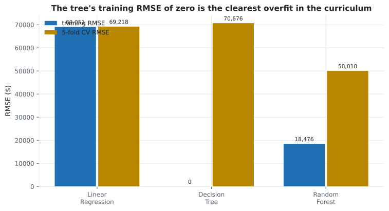
Section titled “Shortlisting models”Train several quickly, cross-validate all of them, and compare the training score against the cross-validated score. That gap is the diagnosis.
from sklearn.ensemble import RandomForestRegressor
from sklearn.linear_model import LinearRegression
from sklearn.metrics import mean_squared_error
from sklearn.model_selection import cross_val_score
from sklearn.pipeline import make_pipeline
from sklearn.tree import DecisionTreeRegressor

candidates = {
    "linear": LinearRegression(),
    "tree": DecisionTreeRegressor(random_state=42),
    "forest": RandomForestRegressor(n_estimators=80, random_state=42, n_jobs=-1),
}

for name, model in candidates.items():
    pipe = make_pipeline(preparation, model)
    pipe.fit(X_train, y_train)
    train_rmse = mean_squared_error(y_train, pipe.predict(X_train)) ** 0.5
    cv_rmse = -cross_val_score(pipe, X_train, y_train, cv=5,
                               scoring="neg_root_mean_squared_error").mean()
    print(f"{name:<7} train {train_rmse:>10,.0f}   cv {cv_rmse:>10,.0f}")

# linear  train     69,051   cv     69,218
# tree    train          0   cv     70,676
# forest  train     18,476   cv     50,010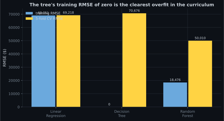
Reading the plot
Section titled “Reading the plot”| Model | Train | CV | Gap | Diagnosis |
|---|---|---|---|---|
| Linear | 69,051 | 69,218 | 167 | Underfitting. No gap at all, and both numbers are high — the model is not flexible enough. |
| Tree | 0 | 70,676 | 70,676 | Overfitting completely. Memorised every row, generalises worse than the linear model. |
| Forest | 18,476 | 50,010 | 31,534 | Overfitting, but useful. A large gap, and still the best CV score by 28%. |
Three lessons in one table:
- A training RMSE of zero is never good news. The tree has one leaf per district.
- No gap is also a warning. Linear regression cannot overfit here because it cannot fit at all; the fix is capacity, not regularisation.
- The forest’s gap says there is more to gain from tuning and from more data — which is exactly what step 7 tries.
Against the 15% expert baseline (roughly $35,530 RMSE from Framing), 50,010 is not yet good enough. That is the number tuning has to move.
Tuning
Section titled “Tuning”GridSearchCV searches the pipeline, so preprocessing choices and model hyperparameters are tuned
together using the double-underscore path:
from sklearn.model_selection import GridSearchCV
from sklearn.pipeline import Pipeline

pipe = Pipeline([
    ("pre", preparation),
    ("rf", RandomForestRegressor(random_state=42, n_jobs=-1)),
])

param_grid = {
    "rf__n_estimators": [30, 100],
    "rf__max_features": [4, 6, 8],
    # Preprocessing is tunable too:
    # "pre__num__imputer__strategy": ["median", "mean"],
}

search = GridSearchCV(pipe, param_grid, cv=3,
                      scoring="neg_root_mean_squared_error", n_jobs=-1)
search.fit(X_train, y_train)

print("best params:", search.best_params_)
# {'rf__max_features': 8, 'rf__n_estimators': 100}
print(f"best CV RMSE: {-search.best_score_:,.0f}")     # 49,821

for mean, params in sorted(zip(-search.cv_results_["mean_test_score"],
                               search.cv_results_["params"]))[:3]:
    print(f"{mean:,.0f}  {params}")
Note that max_features=8 is the largest value in the grid. When the best value sits at the edge
of the grid, the grid was too narrow — extend it and search again. That is a habit worth forming;
it is the most common way a grid search quietly under-delivers.
For large spaces, RandomizedSearchCV samples instead of enumerating, and
RandomizedSearchCV for Large Parameter Spaces
covers when to prefer it.
Error analysis
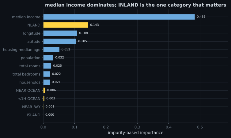
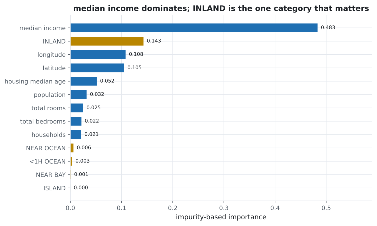
Section titled “Error analysis”A tuned model is not a finished project. Two questions remain: what did it use, and where is it still wrong?
final_model = search.best_estimator_

cat_names = list(final_model.named_steps["pre"]
                 .named_transformers_["cat"].categories_[0])
names = num_attribs + cat_names
importances = final_model.named_steps["rf"].feature_importances_

for name, score in sorted(zip(names, importances), key=lambda p: -p[1]):
    print(f"{name:<22} {score:.4f}")

# median_income          0.4439
# INLAND                 0.1501
# longitude              0.1139
# latitude               0.1025
# housing_median_age     0.0491
# population             0.0385
# total_rooms            0.0298
# total_bedrooms         0.0268
# households             0.0255
# <1H OCEAN              0.0116
# NEAR OCEAN             0.0059
# NEAR BAY               0.0022
# ISLAND                 0.0001
Three actions follow directly:
- Four of the five
ocean_proximitycategories contribute almost nothing. Collapsing them to a singleis_inlandflag would lose about 0.02 of importance and remove four columns. - Latitude and longitude together account for 0.216 — more than every count column combined. An explicit distance-to-city feature is worth trying.
ISLANDscores 0.0001, which is what five rows out of 16,512 buys.
Reading the plot
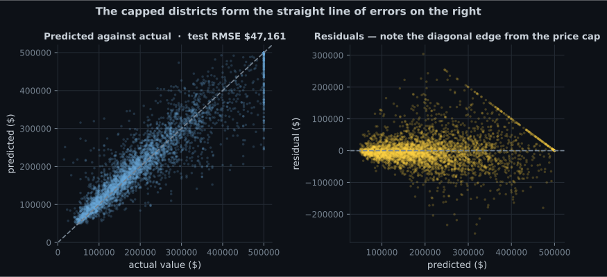
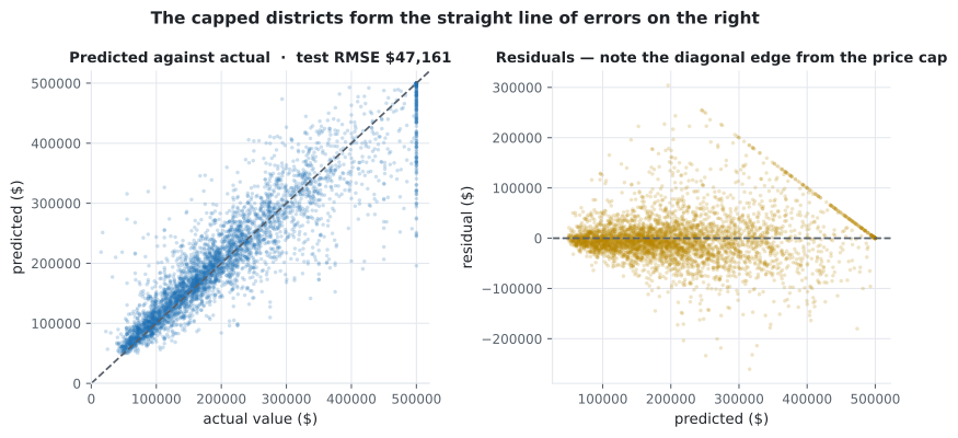
Section titled “Reading the plot”- Predictions compress at both ends. Cheap districts are over-predicted and expensive ones under-predicted — a forest averages leaves, and averages pull toward the middle.
- The horizontal band at the top of the left panel is the capped districts. The model cannot predict above roughly $500k because nothing in training ever was.
- The diagonal edge in the residuals is that same cap, seen from another angle: for a fixed true value, the residual falls exactly one dollar for every dollar the prediction rises.
- Otherwise the residual cloud is shapeless, which is what you want.
The single most valuable next action on this project is not a better model. It is getting real labels for the 965 capped districts.
The test set, once
Section titled “The test set, once”import numpy as np
from scipy import stats
from sklearn.metrics import mean_squared_error
final_model = search.best_estimator_
final_predictions = final_model.predict(X_test)
final_rmse = mean_squared_error(y_test, final_predictions) ** 0.5
print(f"test RMSE: {final_rmse:,.0f}") # 46,768
# A point estimate is not enough — report the interval
squared_errors = (final_predictions - y_test) ** 2
interval = np.sqrt(stats.t.interval(
0.95, len(squared_errors) - 1,
loc=squared_errors.mean(),
scale=stats.sem(squared_errors),
))
print(f"95% CI: [{interval[0]:,.0f}, {interval[1]:,.0f}]")
# 95% CI: [44,832, 48,626]Test RMSE 46,768, with a 95% interval of 44,832 to 48,626.
Two observations, and both matter:
- The test score beats the cross-validated score (46,768 against 49,821). That is fine and not unusual — CV trains on four fifths of the data while the final model trained on all of it. Had the test score been dramatically worse, that would signal overfitting to the CV folds through repeated tuning.
- The interval is roughly ±2,000 wide. A rival model scoring 46,000 is not meaningfully better, and reporting a bare “46,768” invites exactly that false comparison.
Against the $35,530 expert baseline the model still loses. The honest report is: not yet good enough for the stated objective; the largest single obstacle is the capped target, and the next-largest is the absence of a distance-to-city feature.
Ship it
Section titled “Ship it”import joblib
# The pipeline saves preprocessing and model together — one artefact, no drift
joblib.dump(final_model, "california_housing_v1.joblib")
loaded = joblib.load("california_housing_v1.joblib")
print(loaded.predict(X_test.iloc[:3]).round(0)) # raw DataFrame in, prices outWhat to record alongside it:
| Item | Why |
|---|---|
| Metric and interval | 46,768 (44,832–48,626) — the number to compare against later |
| Baselines | Mean 115,393; expert 35,530 |
| Known limits | Cannot predict above $500k; California only |
| Feature importances | Tells you which input to monitor most closely |
| Training data snapshot date | So drift can be measured against something |
| Library versions | A pickled model is not portable across versions |
Then monitor: input distributions, prediction distribution, and — as soon as ground truth arrives — live RMSE against 46,768. Monitoring Model Drift covers the mechanics.
Pitfalls
Section titled “Pitfalls”-
The decision tree scores training RMSE 0 and CV RMSE 70,676, the worst of the three models. What does that mean?
An unpruned tree grows until every leaf is pure, so training error is structurally zero. Only the cross-validated score carries information, and it is the worst of the three.
pch.quizShowAnswer
B — It memorised the training set completely and generalises worse than plain linear regression — An unpruned tree grows until every leaf is pure, so training error is structurally zero. Only the cross-validated score carries information, and it is the worst of the three.
-
Linear regression scores 69,051 training and 69,218 CV — almost no gap. What is the diagnosis?
A tiny gap with a high error means high bias. Regularisation would make it worse; the fix is more capacity or better features.
pch.quizShowAnswer
B — Underfitting: the model is too rigid to fit the data, so there is nothing to overfit and both errors are high — A tiny gap with a high error means high bias. Regularisation would make it worse; the fix is more capacity or better features.
-
The grid search picked max_features=8, the largest value in the grid. What should you do?
The search only found the best value it was offered. When that is the edge value, the grid was too narrow.
pch.quizShowAnswer
B — Widen the grid and search again — a winner at the boundary suggests the true optimum lies outside it — The search only found the best value it was offered. When that is the edge value, the grid was too narrow.
-
Test RMSE is 46,768 with a 95% interval of 44,832 to 48,626. A colleague's model scores 46,100. What can you conclude?
46,100 falls comfortably within 44,832 to 48,626. Declaring a winner on a 668-unit difference is reading noise, which is exactly what reporting the interval prevents.
pch.quizShowAnswer
B — The difference sits well inside the interval, so the two are not distinguishable on this test set — 46,100 falls comfortably within 44,832 to 48,626. Declaring a winner on a 668-unit difference is reading noise, which is exactly what reporting the interval prevents.
🧪 Try It Yourself
Section titled “🧪 Try It Yourself”Exercise 1 – Build the preparation pipeline
Section titled “Exercise 1 – Build the preparation pipeline”Exercise 2 – Read the train-versus-CV gap
Section titled “Exercise 2 – Read the train-versus-CV gap”Exercise 3 – Grid search the pipeline
Section titled “Exercise 3 – Grid search the pipeline”Exercise 4 – Report a confidence interval
Section titled “Exercise 4 – Report a confidence interval”Exercise 5 – Save and reload the whole pipeline
Section titled “Exercise 5 – Save and reload the whole pipeline”- Ten steps, and the first five are the rest of this phase. This page ran shortlist, tune, analyse, evaluate, ship.
- Shortlist by comparing training against cross-validated error: linear 69,051 / 69,218 (underfitting), tree 0 / 70,676 (memorising), forest 18,476 / 50,010 (best, still overfitting).
- Grid search reached CV RMSE 49,821 at
max_features=8— the edge of the grid, so the grid was too narrow. - Importances:
median_income0.444,INLAND0.150, longitude and latitude 0.216 together. Four of five categories are near-worthless. - Test RMSE 46,768, 95% interval 44,832 to 48,626 — one look, no tuning afterwards.
- Still short of the $35,530 expert baseline. The biggest single obstacle is the capped target, not the model.
- Save the whole pipeline, record the baselines and limits, and monitor drift.
Exercise 6 – Simulate the split you did not use
Section titled “Exercise 6 – Simulate the split you did not use”Phase 2 ends here. Continue to Phase 3 - Supervised Learning - Regression — the models used on this page as black boxes, derived from first principles.
pch.coffeeTagline
pch.coffeeCtapch.feedbackHeading
pch.feedbackSubheading