What you’ll learn

• the containment relationship, with real examples in every ring
• that most historical AI contained no machine learning at all
• a measured contest: neural net vs gradient boosting on pixels and on columns
• the data-hunger crossover, measured: logistic 0.8056 vs neural net 0.7630 at n=40
• a decision rule for when deep learning is the right call — and when it is fashion

The nesting

The three terms are not synonyms and they are not rivals. They are nested sets.

Artificial intelligence is the widest: any technique that makes a machine do something we would call intelligent. It is a goal, not a method.

Machine learning is one method for reaching that goal: derive the behaviour from data rather than writing it.

Deep learning is one family of machine-learning models: neural networks with many layers that learn their own feature representations.

figureEvery deep learning system is machine learning; most AI never wasmatplotlib

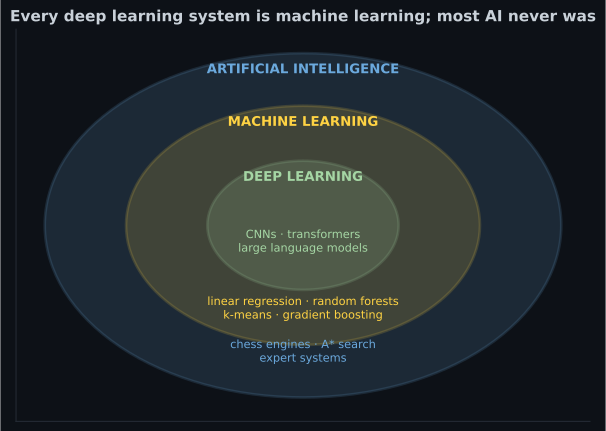
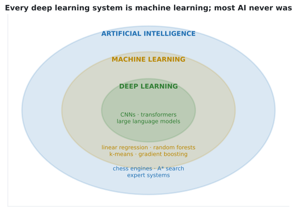
  flowchart TD
  AI["ARTIFICIAL INTELLIGENCE
make machines act intelligently"]
  AI --> S["Symbolic / search AI
rules, logic, planning, A*"]
  AI --> ML["MACHINE LEARNING
derive behaviour from data"]
  ML --> C["Classical ML
you engineer the features"]
  ML --> DL["DEEP LEARNING
the network learns the features"]
  C --> C1["linear + logistic regression
trees, forests, boosting, SVM, k-means"]
  DL --> D1["CNNs, RNNs, transformers
LLMs, diffusion models"]

AI without machine learning

This category is much larger than people expect, and it dominated the field for its first forty years.

None of these improve with experience. Point Mitchell’s definition at them and they fail it immediately: there is no E.

Machine learning without deep learning

Most machine learning in production is not deep learning. Fraud detection, credit scoring, demand forecasting, churn prediction, recommendation ranking — overwhelmingly gradient boosting and logistic regression on structured columns.

The distinguishing feature is who engineers the features. In classical ML, you do: you decide that transactions_per_hourtransactions_per_hour and distance_from_homedistance_from_home are the right columns. In deep learning, the network is handed something close to raw input and constructs its own intermediate representations.

Where deep learning actually wins

The received wisdom is “deep learning wins on unstructured data, classical ML wins on tables”. That is broadly right and worth testing, because the popular version overstates it badly.

Four models, two datasets — 1,797 handwritten digit images (raw pixels) and 1,500 rows of 20 engineered columns:

figureAt this scale there is no deep-learning advantage at allmatplotlib

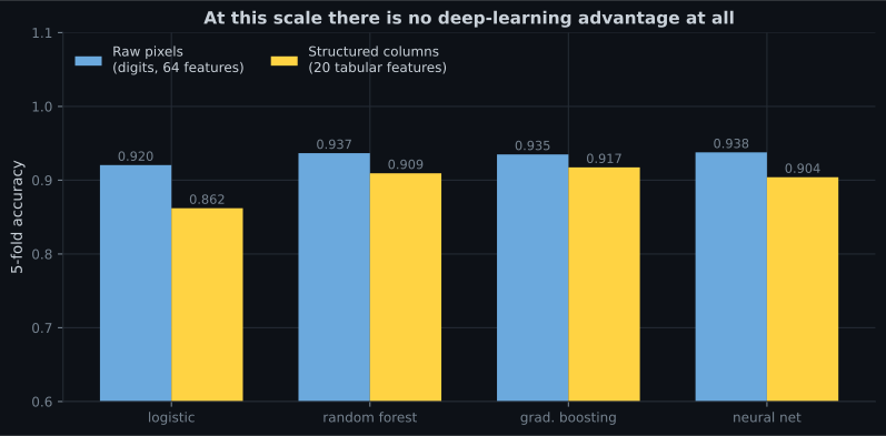
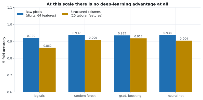
Read that carefully, because it does not say what the slogan says.

On the tabular data the slogan holds: gradient boosting wins at 0.9173, the neural net trails at 0.9040. That is the well-documented result, and it is why Kaggle tabular competitions are won by boosting.

On the pixels the neural net technically wins — by 0.0011 over a random forest. That is not a win, it is a tie. Deep learning’s genuine advantage on images requires convolutional architectures and far more than 1,797 images. At this scale, on this data, there is no deep-learning advantage to be had, and any page that shows you one at this scale is showing you noise.

The data-hunger crossover

The more useful measurement is what happens as data grows. Same digits dataset, same two models, increasing training-set size:

figureThe simpler model wins when data is scarcematplotlib

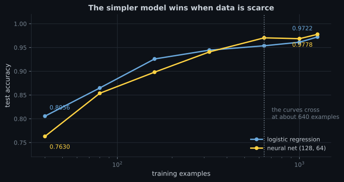
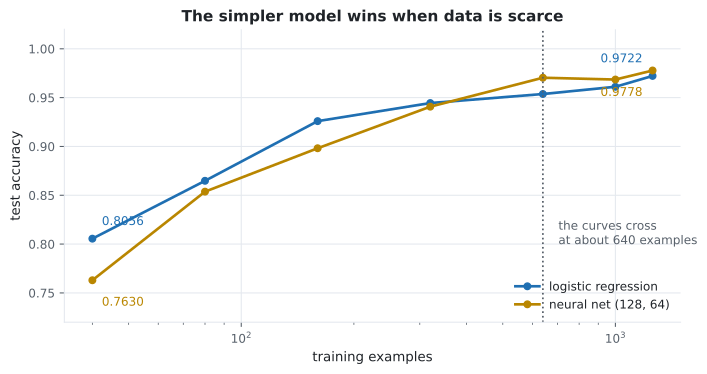
At 40 examples the linear model beats the neural net by 0.0426. The crossover is around 640. And even at full size the neural net’s lead is 0.0056 — real, but small enough that on this problem you would ship the logistic model for its size, speed and interpretability.

This is the durable form of the “deep learning needs data” claim. Not “neural nets are bad on small data” as an insult, but a measured crossover point that depends on your dataset and that you can find yourself in ten lines.

See it move

The sketch plots the two measured columns from the table above on a log axis and sweeps a budget cursor across them. Move the mouse to place the cursor yourself; the panel reports which model is ahead at that training-set size and by how much.

Watch the vertical gap, not the height of the curves. On the left it is wide and blue-side up; it narrows through 320, closes near 640, and then stays open by a hair on the amber side. A model comparison run at a single dataset size only ever samples one slice of this picture — which is why “neural nets beat linear models” and the reverse are both quotable from the same experiment.

Choosing between them

  flowchart TD
  A["What does your input look like?"] --> B{"Rows and columns
you engineered?"}
  B -->|"yes"| C["Gradient boosting first.
Logistic regression as the baseline."]
  B -->|"no — images, audio,
text, video"| D{"How much labelled data?"}
  D -->|"thousands"| E["Fine-tune a pretrained model"]
  D -->|"hundreds of thousands+"| F["Train a deep model"]
  D -->|"hundreds"| G["Pretrained embeddings
+ a classical model on top"]

There is one modern exception worth naming: pretrained models change the arithmetic on small data. You may only have 300 labelled images, but a network trained on millions has already learned the features. Fine-tuning it, or using it purely as a feature extractor and putting logistic regression on top, routinely beats anything classical — because the effective E is not your 300 images, it is the millions the network already saw.

In code

The tabular result, reproducible:

from sklearn.datasets import make_classification
from sklearn.ensemble import HistGradientBoostingClassifier, RandomForestClassifier
from sklearn.linear_model import LogisticRegression
from sklearn.model_selection import cross_val_score
from sklearn.neural_network import MLPClassifier
from sklearn.pipeline import make_pipeline
from sklearn.preprocessing import StandardScaler
 
X, y = make_classification(n_samples=1500, n_features=20, n_informative=8,
                           n_redundant=4, class_sep=1.1, random_state=3)
 
models = {
    "logistic":       make_pipeline(StandardScaler(), LogisticRegression(max_iter=2000)),
    "random forest":  RandomForestClassifier(n_estimators=200, random_state=0),
    "grad boosting":  HistGradientBoostingClassifier(random_state=0),
    "neural net":     make_pipeline(StandardScaler(),
                                    MLPClassifier((128, 64), max_iter=900, random_state=0)),
}
for name, m in models.items():
    print(f"{name:15s} {cross_val_score(m, X, y, cv=5).mean():.4f}")
 
# logistic        0.8620
# random forest   0.9093
# grad boosting   0.9173     <- wins
# neural net      0.9040

from sklearn.datasets import make_classification
from sklearn.ensemble import HistGradientBoostingClassifier, RandomForestClassifier
from sklearn.linear_model import LogisticRegression
from sklearn.model_selection import cross_val_score
from sklearn.neural_network import MLPClassifier
from sklearn.pipeline import make_pipeline
from sklearn.preprocessing import StandardScaler
 
X, y = make_classification(n_samples=1500, n_features=20, n_informative=8,
                           n_redundant=4, class_sep=1.1, random_state=3)
 
models = {
    "logistic":       make_pipeline(StandardScaler(), LogisticRegression(max_iter=2000)),
    "random forest":  RandomForestClassifier(n_estimators=200, random_state=0),
    "grad boosting":  HistGradientBoostingClassifier(random_state=0),
    "neural net":     make_pipeline(StandardScaler(),
                                    MLPClassifier((128, 64), max_iter=900, random_state=0)),
}
for name, m in models.items():
    print(f"{name:15s} {cross_val_score(m, X, y, cv=5).mean():.4f}")
 
# logistic        0.8620
# random forest   0.9093
# grad boosting   0.9173     <- wins
# neural net      0.9040

Finding your own crossover point:

from sklearn.datasets import load_digits
from sklearn.linear_model import LogisticRegression
from sklearn.model_selection import train_test_split
from sklearn.neural_network import MLPClassifier
from sklearn.pipeline import make_pipeline
from sklearn.preprocessing import StandardScaler
 
X, y = load_digits(return_X_y=True)
X_tr, X_te, y_tr, y_te = train_test_split(X, y, test_size=0.3,
                                          random_state=0, stratify=y)
 
for n in (40, 160, 640, len(X_tr)):
    lr = make_pipeline(StandardScaler(), LogisticRegression(max_iter=3000))
    nn = make_pipeline(StandardScaler(),
                       MLPClassifier((128, 64), max_iter=1200, random_state=0))
    lr.fit(X_tr[:n], y_tr[:n])
    nn.fit(X_tr[:n], y_tr[:n])
    print(f"n={n:5d}  logistic {lr.score(X_te, y_te):.4f}"
          f"   neural net {nn.score(X_te, y_te):.4f}")

from sklearn.datasets import load_digits
from sklearn.linear_model import LogisticRegression
from sklearn.model_selection import train_test_split
from sklearn.neural_network import MLPClassifier
from sklearn.pipeline import make_pipeline
from sklearn.preprocessing import StandardScaler
 
X, y = load_digits(return_X_y=True)
X_tr, X_te, y_tr, y_te = train_test_split(X, y, test_size=0.3,
                                          random_state=0, stratify=y)
 
for n in (40, 160, 640, len(X_tr)):
    lr = make_pipeline(StandardScaler(), LogisticRegression(max_iter=3000))
    nn = make_pipeline(StandardScaler(),
                       MLPClassifier((128, 64), max_iter=1200, random_state=0))
    lr.fit(X_tr[:n], y_tr[:n])
    nn.fit(X_tr[:n], y_tr[:n])
    print(f"n={n:5d}  logistic {lr.score(X_te, y_te):.4f}"
          f"   neural net {nn.score(X_te, y_te):.4f}")

Run that on your own data before deciding what you need. It takes a minute and it settles the argument.

Pitfalls

Using the three terms interchangeably. “We’re doing AI” tells a stakeholder nothing. “We fit a gradient-boosted tree on 40 engineered columns” tells them everything.

Assuming deep learning is strictly better. Measured above: gradient boosting beat the neural net on the tabular data (0.9173 vs 0.9040), and logistic regression beat it at every size below 640 examples.

Reading a 0.0011 difference as a win. On the pixel data the top three models spanned 0.0028. Compare against fold-to-fold variance before declaring anything.

Reaching for deep learning on 300 rows. Either use a classical model, or use a pretrained network so the effective experience is millions of examples rather than your 300.

Calling every rule engine “AI” in marketing and then being unable to explain it internally. The nesting diagram is genuinely useful for keeping the conversation honest.

Forgetting that classical ML also needs feature work. Deep learning trades feature engineering for data volume and compute. It is a trade, not a removal.

Recap

• AI ⊃ ML ⊃ deep learning. Chess engines and A* are AI with no learning at all.
• The distinguishing question is who engineers the features: you, or the network.
• On 20 tabular columns, gradient boosting won (0.9173) and the neural net came third (0.9040).
• On 1,797 digit images, the top three models spanned 0.0028 — a tie, not a deep-learning win.
• Logistic regression beat the neural net at every training size up to 320, by 0.0426 at n=40. The curves crossed around 640.
• Pretrained models change the arithmetic: your effective E is what the network already saw.

🧪 Try It Yourself

Exercise 1 – Sort the systems

Exercise 2 – Boosting versus a neural net on columns

Exercise 3 – Find the crossover yourself

Exercise 4 – Is that margin real?

Exercise 5 – Why pretraining is different from re-representing

Exercise 6 – Report the crossover as a decision, not a winner

Next

Types of Machine Learning — the three learning paradigms on one dataset, plus the measurement where a batch model decays from 0.98 to 0.51 while an online one holds at 0.97.