
Cost-Sensitive Learning and Decision Thresholds
What you’ll learn
Section titled “What you’ll learn”- the derivation of the cost-optimal threshold,
- why the default 0.50 cost EUR 12,005 where cost EUR 3,410
- that theory matched a validation-tuned threshold to within EUR 20, with no tuning data
- how wrong your cost estimates can be: any ratio from 21 to 535 stays within 1.4× of optimal
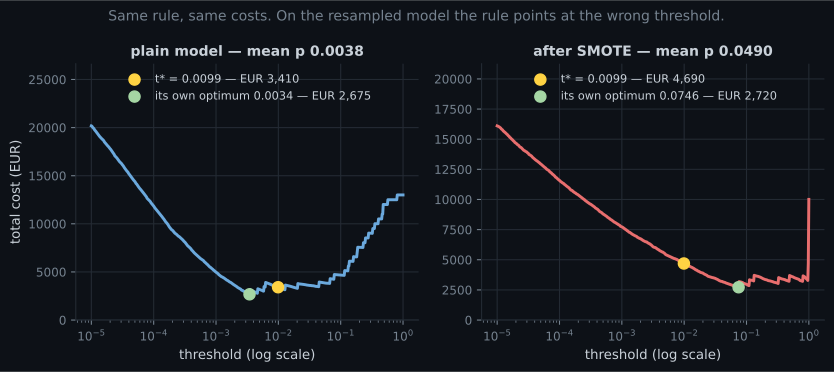
- why a miscalibrated model breaks the rule — a EUR 1,970 penalty after SMOTE
- per-row thresholds when the loss is the transaction amount: 17.8% cheaper, once you have enough frauds to measure it
Where 0.5 comes from, and why it is wrong
Section titled “Where 0.5 comes from, and why it is wrong”predict() thresholds at 0.5. That is the right choice under exactly one assumption: that a false
positive and a false negative cost the same. Almost no real decision satisfies it.
Continuing with the fraud data from the previous page, put two numbers on the errors:
| Error | What it is | Cost |
|---|---|---|
| false positive | an analyst reviews a legitimate transaction | = EUR 5 |
| false negative | a fraud goes through | = EUR 500 |
The split here is 50% to fit, 20% to tune thresholds, 30% to report — 44 frauds to learn from, 17 to tune on, 26 to be judged on.
The derivation
Section titled “The derivation”Take one row with predicted probability . Flagging it costs whenever the row is not fraud; leaving it costs whenever it is:
Flag whenever flagging is cheaper:
That is the whole result. Three properties are worth naming:
- Only the ratio matters. , so doubling both costs changes nothing.
- 0.5 is the special case .
- It requires calibrated probabilities. The comparison is between two expected costs, and if is not a probability the comparison is meaningless. This is where resampling does its damage.
With EUR 5 and EUR 500:
What it is worth
Section titled “What it is worth”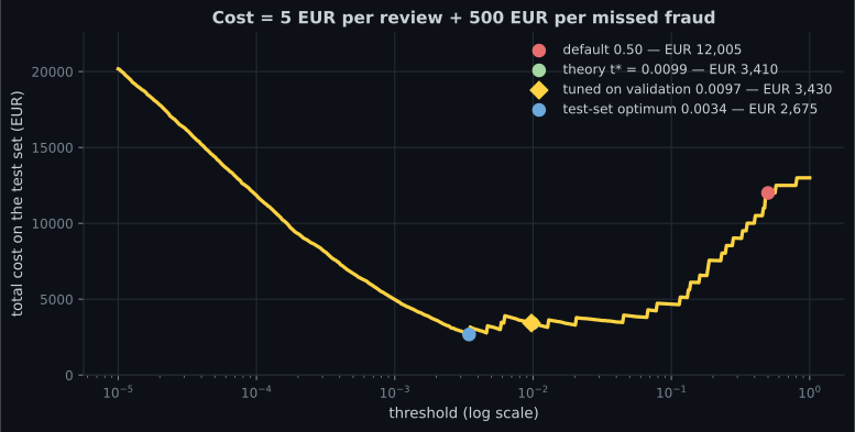
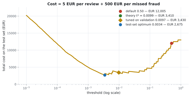
| Policy | Threshold | Alerts | False alerts | Frauds missed | Cost |
|---|---|---|---|---|---|
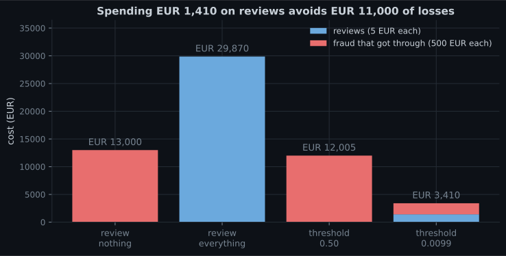
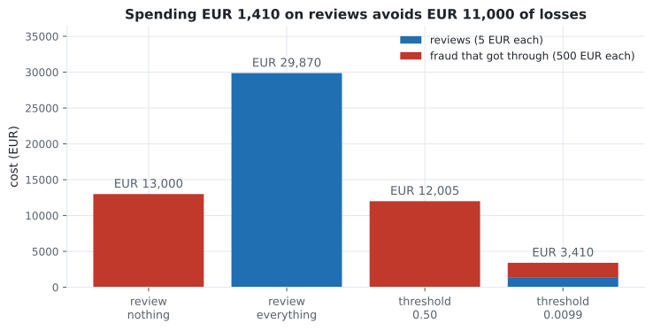
| review nothing | — | 0 | 0 | 26 | EUR 13,000 |
| review everything | 0 | 6,000 | 5,974 | 0 | EUR 29,870 |
| default 0.50 | 0.5000 | 3 | 1 | 24 | EUR 12,005 |
| theory | 0.0099 | 304 | 282 | 4 | EUR 3,410 |
| tuned on validation | 0.0097 | 308 | 286 | 4 | EUR 3,430 |
| test-set optimum (oracle) | 0.0034 | — | — | — | EUR 2,675 |
The comparison to sit with is the third and fourth rows. The same model, the same predictions, and a 3.5× difference in cost. Nothing was retrained; a single number changed.
Two more readings:
Theory beat tuning. The closed form scored EUR 3,410 against the validation-tuned threshold’s EUR 3,430. Not because tuning is wrong in principle, but because tuning on 17 positives is noisy, while the formula uses information tuning cannot see — your actual costs. When you know the costs, compute the threshold; do not search for it.
The oracle is only 22% better. A threshold chosen with knowledge of the test labels reaches EUR 2,675. That gap is the irreducible cost of not knowing which specific rows are fraud, and it is small compared to the 3.5× you lose by leaving the threshold at 0.5.
How precise do the costs have to be?
Section titled “How precise do the costs have to be?”The usual objection is that nobody knows to two decimal places. They do not have to.
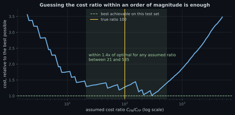
The cost curve is flat-bottomed, so the mapping from cost estimates to money is heavily damped. The practical consequence: do not skip cost-based thresholding because the numbers are uncertain. Ask the business for a range, take the geometric midpoint, and you will land inside the flat region. The mistake that actually costs money is leaving the default in place.
The rule needs calibrated probabilities
Section titled “The rule needs calibrated probabilities”Here is where the previous page’s warning turns into euros. Apply the same to a model trained on SMOTE-resampled data, whose probabilities are inflated roughly 13×:
| Model | Mean | Cost at | Its own best threshold | Its own best cost | Penalty |
|---|---|---|---|---|---|
| plain | 0.0038 | EUR 3,410 | 0.0034 | EUR 2,675 | EUR 735 |
| after SMOTE | 0.0490 | EUR 4,690 | 0.0746 | EUR 2,720 | EUR 1,970 |
The resampled model is not worse at ranking — its achievable cost is within EUR 45 of the plain model’s. It is worse at being a probability, and the rule consumes probabilities. Its optimal threshold has moved from 0.0034 to 0.0746, a factor of 22, purely because of the training prior.
class_weight is the same idea, applied earlier
Section titled “class_weight is the same idea, applied earlier”Passing class_weight={0: 1, 1: 100} multiplies the minority class’s contribution to the loss by the
cost ratio. It is the training-time expression of the same asymmetry, and it moves the decision
boundary rather than the threshold.
# Route 1 — plain model, threshold moved to where the costs say
plain = make_pipeline(StandardScaler(), LogisticRegression(max_iter=3000))
plain.fit(X_fit, y_fit)
flag = plain.predict_proba(X_test)[:, 1] >= C_FP / (C_FP + C_FN)

# Route 2 — weighted training, threshold left at 0.5
weighted = make_pipeline(
    StandardScaler(),
    LogisticRegression(max_iter=3000, class_weight={0: 1, 1: C_FN / C_FP}))
weighted.fit(X_fit, y_fit)
flag = weighted.predict(X_test)
Prefer route 1, for three reasons that have nothing to do with accuracy:
- The threshold is a deployment parameter. Costs change — a new fraud pattern, a cheaper review team, a seasonal spike — and route 1 changes a config value while route 2 retrains.
- Route 1 keeps calibrated probabilities, so you can also report expected loss per transaction.
- One model can serve several decisions at once: a high threshold for automatic blocking, a low one for manual review, from the same probabilities.
Use class_weight when the minority class is so rare that the optimiser barely notices it, or when a
library gives you no access to probabilities.
When the loss is not a constant
Section titled “When the loss is not a constant”Missing a EUR 2 fraud and missing a EUR 900 fraud are not the same event, and the derivation never required to be constant. Redo it per row with :
Cheap transactions get a high bar; expensive ones get a low one. On this data the amounts are lognormal across the whole dataset with a median of EUR 24.55, a mean of EUR 39.70 and a maximum of EUR 1,103.67. On the test split that makes the per-row thresholds span 0.0056 to 0.8662, with a median of 0.1694.
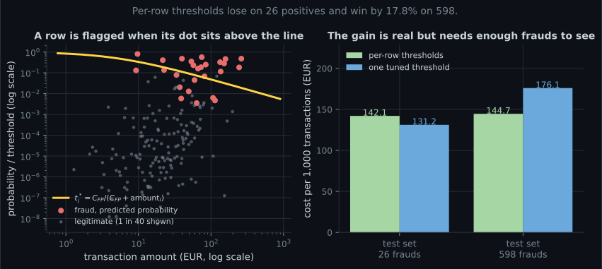
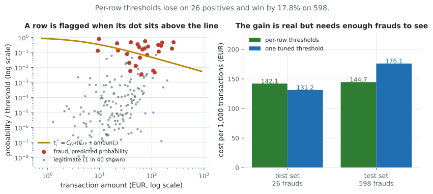
| Test set | Frauds | Per-row thresholds | One tuned threshold | Difference |
|---|---|---|---|---|
| 6,000 rows | 26 | EUR 853 | EUR 787 | 8.3% worse |
| 120,000 rows | 598 | EUR 17,361 | EUR 21,128 | 17.8% better |
This is the most useful measurement on the page, and it says two things at once.
The theory is right. With enough positives, per-row thresholds save 17.8% — 1,740 alerts catching 384 of 598 frauds, against 1,594 alerts catching 400 of them. Fewer frauds caught, less money lost: the ones it lets through are the cheap ones.
Your test set probably cannot see it. At 26 positives, a 15% effect is far below the noise floor; one unlucky EUR 250 fraud moves the total by more than the entire effect. If you evaluate a per-row-threshold change on a handful of positives and it looks worse, you have learned nothing about the change.
See it move
Section titled “See it move”Two costs, one threshold, and the expected cost per transaction. The curve below is computed in closed form from the fraud and legitimate score distributions, so you can watch track the ratio.
Drag the cost of a missed fraud from EUR 5 to EUR 10,000 and watch two things: the minimum slides
left, monotonically, and the threshold it corresponds to is always . At
the minimum sits exactly where predict() would put it — which is the only setting
in which the default is defensible.
Putting it together
Section titled “Putting it together” flowchart TD
A["A model that outputs
probabilities"] --> B{"Are they calibrated?"}
B -->|"resampled or
class-weighted"| C["Recalibrate, or tune the
threshold empirically"]
B -->|"yes"| D["Get C_FP and C_FN
from the business"]
D --> E{"Is the loss
row-dependent?"}
E -->|"no"| F["t* = C_FP / (C_FP + C_FN)"]
E -->|"yes — an amount,
a lifetime value"| G["t*_i = C_FP / (C_FP + loss_i)"]
F --> H["Report cost, alerts,
recall at that threshold"]
G --> H
C --> H
H --> I["Re-derive when the costs
change. Do not retrain."]
Pitfalls
Section titled “Pitfalls”| Pitfall | Why it bites | What to do |
|---|---|---|
| Leaving the threshold at 0.5 | EUR 12,005 against EUR 3,410 on identical predictions | Derive it from costs, or tune it, but never inherit it |
| Applying to resampled probabilities | EUR 1,970 penalty after SMOTE | Recalibrate, or tune empirically |
| Refusing to threshold because costs are uncertain | Any ratio from 21 to 535 stays within 1.4× | Ask for a range, take the middle, ship |
| Retraining when costs change | The threshold is a config value | Keep the model, move the threshold |
| Using one threshold when the loss varies per row | 17.8% of avoidable cost at scale | |
| Comparing policies on a handful of positives | Per-row thresholds looked 8.3% worse on 26 frauds | Bootstrap the cost difference before concluding |
| Optimising F1 and calling it cost-sensitive | F1 encodes a cost ratio of 1 that nobody chose | State the ratio you are assuming, explicitly |
- , derived by comparing two expected costs per row.
- At EUR 5 and EUR 500 that is 0.009901, and it cost EUR 3,410 against the default’s EUR 12,005 — a 3.5× difference from one number.
- A threshold tuned on 17 validation positives scored EUR 3,430: the closed form did marginally better with no data.
- The oracle threshold reached EUR 2,675, so the remaining headroom is 22%.
- Any assumed cost ratio between 21 and 535 stays within 1.4× of optimal. Precision is not required; using 0.5 is.
- The rule needs calibrated probabilities: after SMOTE it costs EUR 4,690 against that model’s own achievable EUR 2,720.
- Per-row thresholds were 17.8% cheaper on 598 frauds and 8.3% worse on 26 — the theory is right and small test sets cannot see it.
-
A review costs EUR 5 and a missed fraud costs EUR 500. What threshold should you flag at?
5 / 505 = 0.009901. On the measured test set that cost EUR 3,410 against EUR 12,005 at the default, using the very same predictions. Tuning on validation independently arrived at 0.0097 and scored EUR 3,430.
pch.quizShowAnswer
B — 0.0099 — that is C_FP / (C_FP + C_FN), the point where the expected cost of flagging equals the expected cost of passing — 5 / 505 = 0.009901. On the measured test set that cost EUR 3,410 against EUR 12,005 at the default, using the very same predictions. Tuning on validation independently arrived at 0.0097 and scored EUR 3,430.
-
You do not know C_FN precisely — somewhere between EUR 100 and EUR 1,500 per missed fraud. What now?
The cost curve is flat-bottomed: a factor of 25 in the assumed ratio maps to 40% in cost. The default 0.5 corresponds to an assumed ratio of 1, which on this data costs 3.5x the optimum. Uncertainty is not a reason to keep the worst option.
pch.quizShowAnswer
B — Pick a value in the middle and ship it — any assumed cost ratio between 21 and 535 lands within 1.4x of the best achievable cost — The cost curve is flat-bottomed: a factor of 25 in the assumed ratio maps to 40% in cost. The default 0.5 corresponds to an assumed ratio of 1, which on this data costs 3.5x the optimum. Uncertainty is not a reason to keep the worst option.
-
Your model was trained with SMOTE and its mean predicted probability is 0.0490 against a true rate of 0.0044. You apply t* = 0.0099. What happens?
Resampling shifts the prior, so every probability is inflated — here about 13-fold. The ranking is fine, but the closed form consumes probabilities, and feeding it inflated ones moves the decision to the wrong place. Recalibrate or tune empirically.
pch.quizShowAnswer
B — You over-flag: the rule assumes calibrated probabilities, and the cost comes out at EUR 4,690 against the EUR 2,720 that same model could reach at 0.0746 — Resampling shifts the prior, so every probability is inflated — here about 13-fold. The ranking is fine, but the closed form consumes probabilities, and feeding it inflated ones moves the decision to the wrong place. Recalibrate or tune empirically.
-
Why prefer moving the threshold over training with class_weight?
Both express the same asymmetry and reach similar operating points. The difference is operational: a config change against a retrain, and calibrated probabilities against distorted ones. Reach for class_weight when the optimiser genuinely ignores the minority class, or when a library hides predict_proba.
pch.quizShowAnswer
B — The threshold is a deployment parameter: costs change without retraining, probabilities stay calibrated, and one model can serve several decisions at once — Both express the same asymmetry and reach similar operating points. The difference is operational: a config change against a retrain, and calibrated probabilities against distorted ones. Reach for class_weight when the optimiser genuinely ignores the minority class, or when a library hides predict_proba.
-
Per-row thresholds looked 8.3% worse than a single tuned threshold on your 26-positive test set. What is the right conclusion?
With rare, high-variance losses the noise floor is enormous. One EUR 250 fraud is worth 50 unnecessary reviews, so a 15% systematic effect is invisible on 26 positives. Bootstrap the cost difference and report 'no measurable difference' rather than 'worse'.
pch.quizShowAnswer
B — The test set cannot resolve the effect — the same rule was 17.8% cheaper on a test set with 598 frauds, and at 26 positives one unlucky expensive fraud dominates the total — With rare, high-variance losses the noise floor is enormous. One EUR 250 fraud is worth 50 unnecessary reviews, so a 15% systematic effect is invisible on 26 positives. Bootstrap the cost difference and report 'no measurable difference' rather than 'worse'.
🧪 Try It Yourself
Section titled “🧪 Try It Yourself”Exercise 1 – Derive and apply the threshold
Section titled “Exercise 1 – Derive and apply the threshold”Exercise 2 – Beat the tuner with arithmetic
Section titled “Exercise 2 – Beat the tuner with arithmetic”Exercise 3 – Map the sensitivity to your cost guess
Section titled “Exercise 3 – Map the sensitivity to your cost guess”Exercise 4 – Price the miscalibration
Section titled “Exercise 4 – Price the miscalibration”Exercise 5 – Give every row its own threshold
Section titled “Exercise 5 – Give every row its own threshold”Time Series Forecasting Fundamentals — every split so far has been random. When rows are ordered in time, a random split leaks the future into the past, and the measured penalty is large.
pch.coffeeTagline
pch.coffeeCtapch.feedbackHeading
pch.feedbackSubheading