MAP Estimation and Model Fitting

Page 804 ended on the book’s own warning: “especially in the ‘small’ data regime, maximum likelihood estimation can lead to overfitting.” Maximum likelihood has no mechanism to prevent this — it maximises fit to the data it has and stops.

§8.2.3 solved the same problem by adding a penalty. §8.3.2 solves it by adding a prior. The book calls the two ideas analogous. They are the same estimator, and this page measures the equality to $1.2\times10^{-14}$.

What you’ll learn

• Equations 8.19 and 8.20: Bayes’ theorem applied to parameters, and why the denominator can be dropped.
• What MAP estimation is, and the sense in which it “bridges the non-probabilistic and probabilistic worlds”.
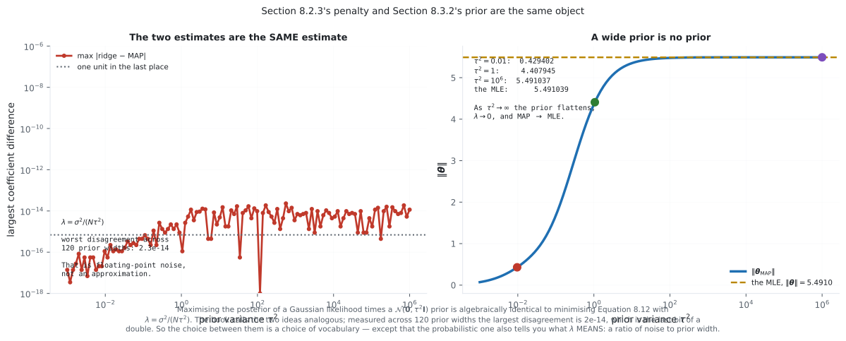
• The exact correspondence: a $\mathcal{N}(\mathbf{0}, \tau^2\mathbf{I})$ prior gives ridge regression with $\lambda = \sigma^2/(N\tau^2)$, measured to $1.2\times10^{-14}$ across six orders of magnitude of prior width.
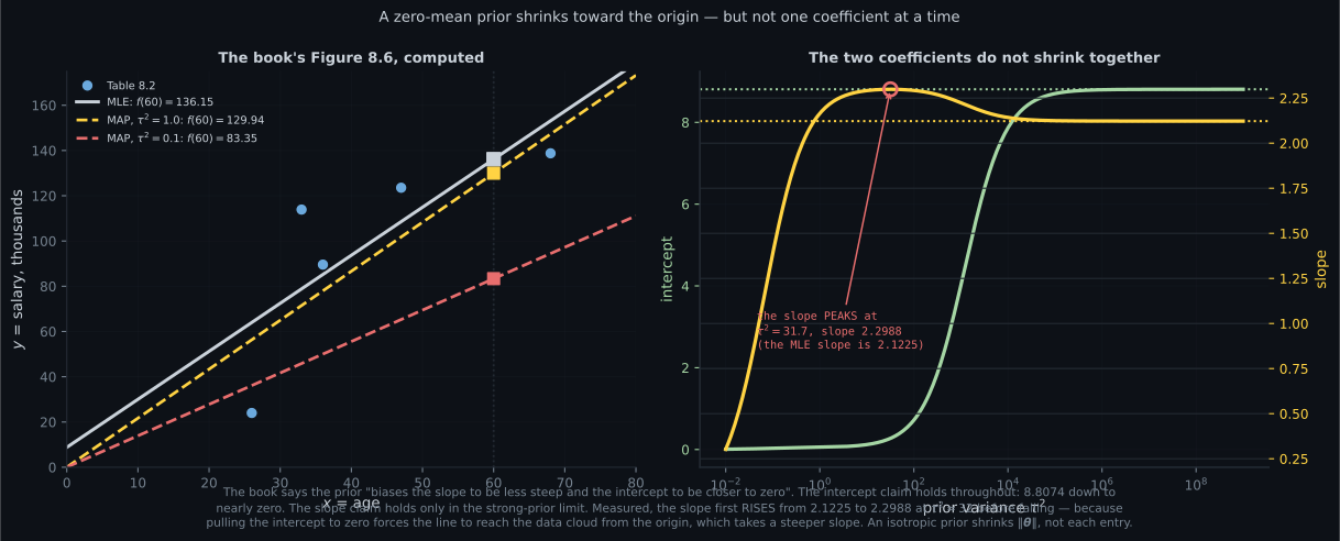
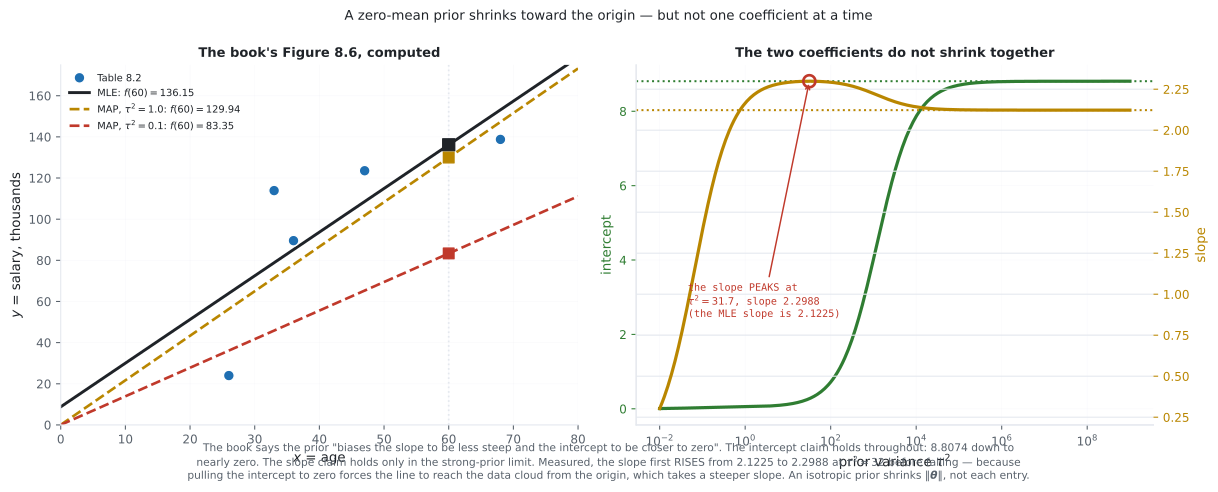
• Why the book’s phrase “the prior biases the slope to be less steep” needs a caveat — measured, the slope first gets steeper, peaking at $2.2988$ against an MLE slope of $2.1225$.
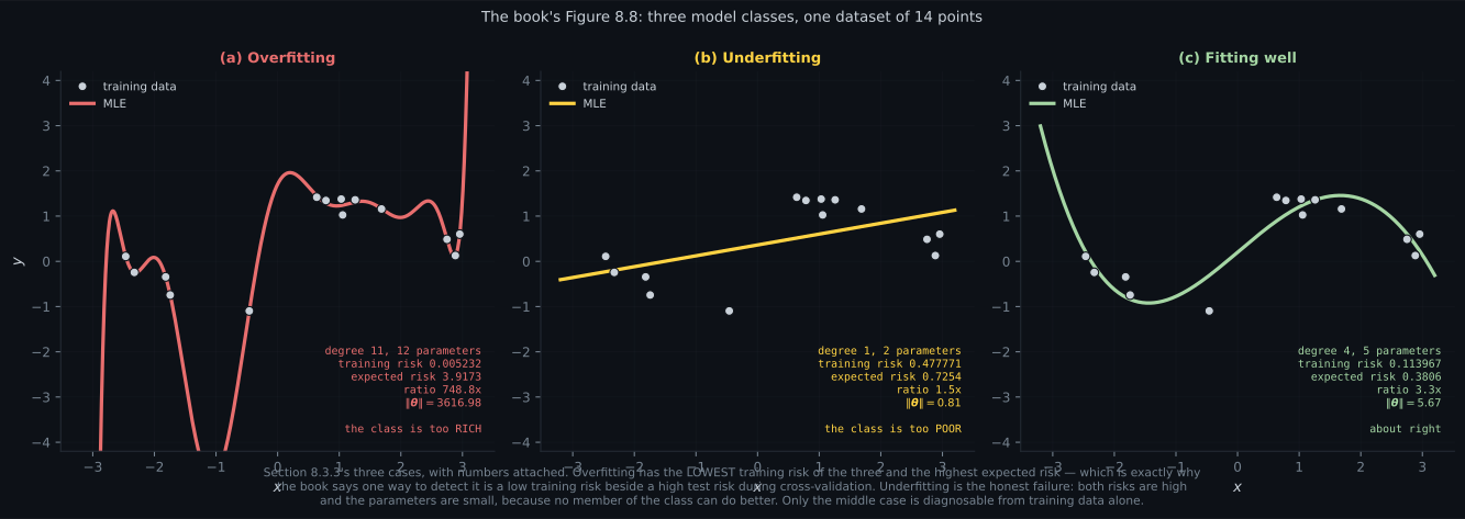
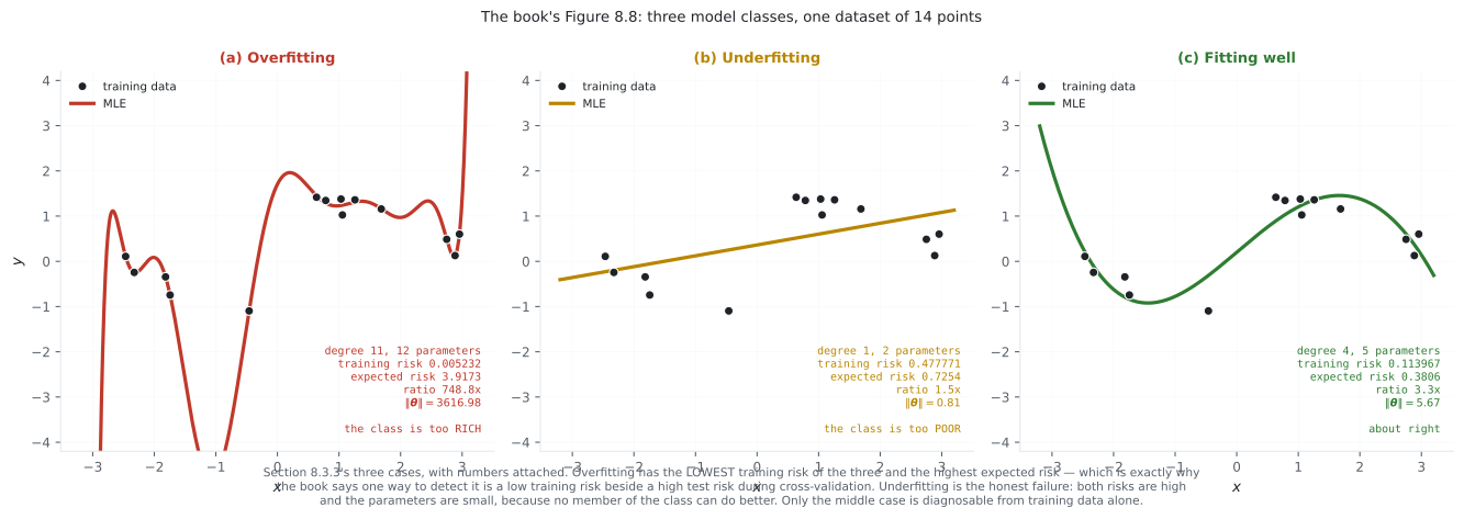
• §8.3.3’s three cases from Figure 8.8, with risks attached: overfitting has the lowest training risk of the three and a $748.8\times$ ratio.
• §8.3.4: what happens when you put a nonlinear function on a linear predictor, and where that leads.

Intuition: an opinion held before the data arrives

Maximum likelihood asks which parameter best explains the data? If the data is thin, the answer can be absurd — a degree-11 polynomial through 14 points with coefficients in the thousands “explains” the data beautifully.

A prior is an opinion you hold before seeing anything. Not “the coefficients are zero” — an opinion that strong would ignore the data entirely — but “coefficients near zero are more plausible than coefficients in the thousands.” The posterior combines that opinion with the evidence, and the maximum of the posterior is a compromise.

The compromise is governed by one ratio: how noisy is the data, against how confident is the opinion? That ratio is $\sigma^2/\tau^2$, and it is exactly $\lambda$ up to the factor $N$. Noisy data or a confident prior means shrink hard; clean data or a vague prior means trust the likelihood.

diagram Two vocabularies, one estimator mermaid

  flowchart TD
  ERM["Section 8.2: minimise
R_emp + lambda ||theta||^2"]
  PROB["Section 8.3: maximise
p(y | theta) p(theta)"]
  ERM --> SAME["the SAME theta
measured to 1.2e-14"]
  PROB --> SAME
  SAME --> L["with lambda = sigma^2 / (N tau^2)"]
  L --> M1["noisy data, big sigma: shrink harder"]
  L --> M2["confident prior, small tau: shrink harder"]
  L --> M3["more data, big N: shrink less"]
  PROB -.->|"but only the point estimate"| PT["MAP is still ONE number
the full posterior is Section 8.4"]
  style PT stroke-dasharray: 4 3

§8.3.2 Maximum a posteriori estimation

If we have prior knowledge about the distribution of $\boldsymbol\theta$, we multiply an extra term onto the likelihood. Bayes’ theorem (§6.3) gives the update:

$$p(\boldsymbol\theta \mid \mathbf{x}) = \frac{p(\mathbf{x} \mid \boldsymbol\theta)\,p(\boldsymbol\theta)}{p(\mathbf{x})}$$

with the three named pieces: the posterior $p(\boldsymbol\theta \mid \mathbf{x})$, the prior $p(\boldsymbol\theta)$, and the likelihood $p(\mathbf{x} \mid \boldsymbol\theta)$ “that links the parameters $\boldsymbol\theta$ and the observed data $\mathbf{x}$”.

Since $p(\mathbf{x})$ does not depend on $\boldsymbol\theta$, it cannot affect the maximisation:

$$p(\boldsymbol\theta \mid \mathbf{x}) \propto p(\mathbf{x} \mid \boldsymbol\theta)\,p(\boldsymbol\theta)$$

The book’s note on why that matters practically: “The preceding proportion relation hides the density of the data $p(\mathbf{x})$, which may be difficult to estimate.” It is an integral over all of parameter space, and §8.4 will need it — but MAP does not.

So instead of minimising the negative log-likelihood, minimise the negative log-posterior. That is maximum a posteriori estimation.

Example 8.6, and the exact correspondence

The book’s example: assume $p(\boldsymbol\theta) = \mathcal{N}(\mathbf{0}, \boldsymbol\Sigma)$, and note that “the conjugate prior of a Gaussian is also a Gaussian (§6.6.1), and therefore we expect the posterior distribution to also be a Gaussian”.

Take $\boldsymbol\Sigma = \tau^2\mathbf{I}$ and write out the negative log-posterior:

$$-\log p(\boldsymbol\theta \mid \mathbf{y}) = \underbrace{\frac{1}{2\sigma^2}\sum_{n}(y_n - \mathbf{x}_n^\top\boldsymbol\theta)^2}_{\text{from the likelihood}} + \underbrace{\frac{1}{2\tau^2}\lVert\boldsymbol\theta\rVert^2}_{\text{from the prior}} + \text{const}$$

Multiply through by $2\sigma^2/N$ — a positive constant, so the minimiser is unchanged:

$$\frac{1}{N}\sum_{n}(y_n - \mathbf{x}_n^\top\boldsymbol\theta)^2 + \frac{\sigma^2}{N\tau^2}\lVert\boldsymbol\theta\rVert^2$$

That is Equation 8.12 exactly, with

$$\boxed{\ \lambda = \frac{\sigma^2}{N\tau^2}\ }$$

Measured across six orders of magnitude

$\tau^2$	$\lambda = \sigma^2/(N\tau^2)$	max $\lvert$ridge $-$ MAP$\rvert$	$\lVert\boldsymbol\theta\rVert$
$0.01$	$4.900\times10^{-1}$	$1.39\times10^{-17}$	$0.439975$
$0.1$	$4.900\times10^{-2}$	$6.66\times10^{-16}$	$1.677835$
$1$	$4.900\times10^{-3}$	$2.22\times10^{-15}$	$4.357258$
$10$	$4.900\times10^{-4}$	$1.24\times10^{-14}$	$5.350205$
$10^3$	$4.900\times10^{-6}$	$2.66\times10^{-15}$	$5.489592$
$10^6$	$4.900\times10^{-9}$	$1.15\times10^{-14}$	$5.491037$

The MLE has $\lVert\boldsymbol\theta\rVert = 5.491039$. As $\tau^2 \to \infty$ the prior flattens, $\lambda \to 0$, and MAP becomes MLE.

The worst disagreement anywhere is $1.24\times10^{-14}$, which is floating-point noise. These are not similar estimators; they are the same estimator computed two ways.

What the probabilistic vocabulary buys, given that the answer is identical: it tells you what $\lambda$ means. In §8.2.3, $\lambda$ is a knob you tune by cross-validation with no units and no interpretation. Here it is $\sigma^2/(N\tau^2)$ — a ratio of noise variance to prior variance, divided by the sample size. That immediately explains three behaviours: noisier data shrinks harder, a more confident prior shrinks harder, and more data shrinks less.

What MAP still does not give you

The book is precise about the limit: MAP “can be considered to bridge the non-probabilistic and probabilistic worlds as it explicitly acknowledges the need for a prior distribution but it still only produces a point estimate of the parameters.”

You wrote down a whole posterior distribution and then threw all of it away except the location of its peak. §8.4 is what happens when you keep the rest.

The book’s own phrasing about the slope needs a caveat

Figure 8.6’s caption says the prior “biases the slope to be less steep and the intercept to be closer to zero”. Measured on Table 8.2’s five points, the intercept claim holds throughout — but the slope claim holds only in the strong-prior limit:

$\tau^2$	intercept	slope	$f(60)$
MLE	$8.8074$	$2.1225$	$136.15$
$10^3$	$4.0151$	$2.2240$	$137.46$
$100$	$0.7184$	$2.2926$	$138.28$
$31.71$	$0.2729$	$\mathbf{2.2988}$	$138.20$
$10$	$0.1206$	$2.2916$	$137.62$
$1$	$0.0532$	$2.1648$	$129.94$
$0.1$	$0.0302$	$1.3887$	$83.35$

The slope first gets steeper, peaking at $2.2988$ against an MLE slope of $2.1225$, and only drops below the MLE once $\tau^2 < 1$.

The reason is geometric. An isotropic prior shrinks $\lVert\boldsymbol\theta\rVert$, not each coefficient individually. The intercept is cheap to shrink because the data barely constrains it — but pulling the line’s $y$-intercept toward zero while it must still pass through a data cloud centred at age $42$ forces a steeper slope. The two coefficients trade against each other.

This is the practical reason to centre your inputs and exclude the intercept from the penalty, as page 801 noted from the other direction.

§8.3.3 Model fitting

“Fitting” means optimising parameters to minimise a loss. The parametrisation defines a model class $M_{\boldsymbol\theta}$; the data comes from some unknown $M^*$; and you search within $M_{\boldsymbol\theta}$ for whatever is closest to $M^*$.

Figure 8.7’s picture is worth holding: a circle $M_{\boldsymbol\theta}$ representing everything your class can express, a point $M^*$ outside it, and a search that starts at $M_{\boldsymbol\theta_0}$ and ends at $M_{\boldsymbol\theta^*}$ — the closest point in the circle, which is still not $M^*$.

Three outcomes, and the book gives each a crisp characterisation:

Overfitting — the class is too rich. ”$M_{\boldsymbol\theta}$ could model much more complicated datasets.” The flexible class “uses all its modeling power to reduce the training error. If the training data is noisy, it will therefore find some useful signal in the noise itself.” Models that overfit “typically have a large number of parameters”.

Underfitting — the class is not rich enough. If the data is sinusoidal and your class is straight lines, “the best optimization procedure will not get us close to the true model”. Models that underfit “typically have few parameters”.

Fitting well — “the parametrized model class is about right”.

Measured on 14 points, reproducing Figure 8.8’s three panels:

case	degree	training risk	expected risk	ratio	$\lVert\boldsymbol\theta\rVert$
(a) overfitting	$11$	$\mathbf{0.005232}$	$3.9173$	$748.8\times$	$3616.98$
(b) underfitting	$1$	$0.477771$	$0.7254$	$1.5\times$	$0.81$
(c) fitting well	$4$	$0.113967$	$\mathbf{0.3806}$	$3.3\times$	$5.67$

Read the training-risk column. Overfitting has the lowest training risk of the three — by a factor of $22$ over the good model — and the worst expected risk. That is exactly why the book’s margin note says: “One way to detect overfitting in practice is to observe that the model has low training risk but high test risk during cross validation.”

And note the asymmetry. Underfitting is visible from training data alone: a training risk of $0.478$ with only two parameters is obviously poor. Overfitting is invisible from training data alone — every number looks excellent.

The book’s closing advice for the rich-model case, which is the normal case in practice: “To mitigate the problem of overfitting, we can use regularization (§8.2.3) or priors (§8.3.2).” This page has just shown those are the same thing.

§8.3.4 Further reading

Two pointers worth carrying. First, maximum likelihood “generalizes the idea of least-squares regression for linear models”, developed in Chapter 9. Second, restricting the predictor to a linear form with a nonlinear function $\phi$ applied to the output:

$$p(y_n \mid \mathbf{x}_n, \boldsymbol\theta) = \phi(\boldsymbol\theta^\top\mathbf{x}_n)$$

opens up “other models for other prediction tasks, such as binary classification or modeling count data” (McCullagh and Nelder, 1989). That is the generalized linear model, and the machinery is the exponential family of §6.6.

Worked example by hand

MAP for a Gaussian mean — the smallest case where the shrinkage is visible.

Model: $y_n \sim \mathcal{N}(\theta, \sigma^2)$ with $N$ observations, and prior $\theta \sim \mathcal{N}(0, \tau^2)$.

Step 1: the negative log-posterior. Dropping terms free of $\theta$:

$$-\log p(\theta \mid \mathbf{y}) = \frac{1}{2\sigma^2}\sum_{n=1}^{N}(y_n - \theta)^2 + \frac{\theta^2}{2\tau^2} + \text{const}$$

Step 2: differentiate and set to zero.

$$-\frac{1}{\sigma^2}\sum_{n=1}^{N}(y_n - \theta) + \frac{\theta}{\tau^2} = 0$$ $$\frac{N\theta}{\sigma^2} + \frac{\theta}{\tau^2} = \frac{1}{\sigma^2}\sum_{n=1}^{N}y_n$$

Step 3: solve. Multiply by $\sigma^2$ and write $\bar{y}$ for the sample mean:

$$\theta\left(N + \frac{\sigma^2}{\tau^2}\right) = N\bar{y} \quad\Longrightarrow\quad \boxed{\ \hat\theta_{\text{MAP}} = \frac{N}{N + \sigma^2/\tau^2}\,\bar{y}\ }$$

Step 4: read it. The MAP estimate is the sample mean shrunk toward zero by the factor $\dfrac{N}{N + \sigma^2/\tau^2}$, which is always in $(0, 1)$. And the three limits are all the right ones:

limit	shrinkage factor	estimate	reading
$\tau^2 \to \infty$	$\to 1$	$\bar{y}$, the MLE	a vague prior is no prior
$\tau^2 \to 0$	$\to 0$	$0$	a certain prior ignores the data
$N \to \infty$	$\to 1$	$\bar{y}$	data eventually wins
$\sigma^2 \to \infty$	$\to 0$	$0$	useless data, trust the prior

Step 5: connect it. Write $\lambda = \sigma^2/(N\tau^2)$ and the factor becomes $\dfrac{1}{1 + \lambda}$ — precisely the $\theta(\lambda) = 1/(1+\lambda)$ that page 803’s worked example derived from the penalty side, with no probability anywhere. Two derivations, two vocabularies, one formula.

See it move

The equality is the thing to feel. Drag the prior and the penalty and watch them land on the same answer:

sketch One knob, two names p5.js Pause Restart

The same estimate computed twice — once as ridge regression with a penalty lambda, once as MAP with a Gaussian prior of variance tau squared. Drag either knob and the other follows through lambda equals sigma squared over N tau squared. The two fitted curves are drawn on top of each other; they never separate.

From scratch

map_estimation.py

import numpy as np
 
SIGMA = 0.35
 
def make(n, seed, noise=SIGMA):
    rng = np.random.default_rng(seed)
    x = np.sort(rng.uniform(-3, 3, n))
    return x, np.sin(1.4 * x) + 0.3 * x + noise * rng.standard_normal(n)
 
x, y = make(25, seed=3)
Phi = np.vander(x / 3.0, 4, increasing=True)
N, D = Phi.shape
 
def ridge(lam):
    """Section 8.2.3, Equation 8.12."""
    return np.linalg.solve(Phi.T @ Phi / N + lam * np.eye(D), Phi.T @ y / N)
 
def map_estimate(tau2):
    """Section 8.3.2: maximise a Gaussian likelihood times a N(0, tau2 I) prior."""
    return np.linalg.solve(Phi.T @ Phi / SIGMA ** 2 + np.eye(D) / tau2,
                           Phi.T @ y / SIGMA ** 2)
 
mle = np.linalg.lstsq(Phi, y, rcond=None)[0]
print(f"N = {N}, sigma = {SIGMA}, so sigma^2 = {SIGMA ** 2:.6f}")
print("\nthe correspondence is lambda = sigma^2 / (N tau^2):\n")
print(f"{'tau^2':>10} {'lambda':>13} {'max |ridge - MAP|':>19} "
      f"{'||theta||':>12}")
worst = 0.0
for t2 in (0.01, 0.1, 1.0, 10.0, 1e3, 1e6):
    lam = SIGMA ** 2 / (N * t2)
    d = float(np.abs(ridge(lam) - map_estimate(t2)).max())
    worst = max(worst, d)
    print(f"{t2:>10.4g} {lam:>13.3e} {d:>19.2e} "
          f"{np.linalg.norm(map_estimate(t2)):>12.6f}")
print(f"\nworst disagreement: {worst:.2e}  -- floating-point noise")
print(f"the MLE has ||theta|| = {np.linalg.norm(mle):.6f}")
print("as tau^2 grows the prior flattens, lambda -> 0, and MAP -> MLE")
 
# --- Figure 8.6 on the book's own five points ---------------------------
print("\n--- the book's Figure 8.6, on Table 8.2 -----------------------")
AGE = np.array([36.0, 47.0, 26.0, 68.0, 33.0])
SAL = np.array([89.563, 123.543, 23.989, 138.769, 113.888])
X = np.column_stack([np.ones_like(AGE), AGE])
mle5 = np.linalg.lstsq(X, SAL, rcond=None)[0]
r5 = SAL - X @ mle5
s2 = float(r5 @ r5 / len(SAL))
 
def map5(tau2):
    return np.linalg.solve(X.T @ X / s2 + np.eye(2) / tau2, X.T @ SAL / s2)
 
print(f"MLE          : intercept {mle5[0]:9.4f}  slope {mle5[1]:.4f}  "
      f"f(60) = {mle5 @ [1, 60.0]:.2f}")
for t2 in (1e9, 1e3, 100.0, 31.71, 10.0, 1.0, 0.1):
    m = map5(t2)
    print(f"tau^2 = {t2:>8.4g}: intercept {m[0]:9.4f}  slope {m[1]:.4f}  "
          f"f(60) = {m @ [1, 60.0]:.2f}")
 
t2s = np.geomspace(1e-2, 1e9, 400)
slopes = np.array([map5(t)[1] for t in t2s])
k = int(np.argmax(slopes))
print(f"\nthe book says the prior biases the slope to be LESS steep.")
print(f"measured: the slope first RISES, peaking at {slopes[k]:.4f} at "
      f"tau^2 = {t2s[k]:.4g},")
print(f"against an MLE slope of {mle5[1]:.4f}. It falls below the MLE only")
print("once the prior is tight enough to matter -- an isotropic prior")
print("shrinks ||theta||, not each coefficient separately.")
 
# --- Section 8.3.3: the three cases ------------------------------------
print("\n--- Section 8.3.3, Figure 8.8's three cases -------------------")
xtr, ytr = make(14, seed=21)
xte, yte = make(4000, seed=99)
print(f"{'case':>16} {'degree':>7} {'train risk':>13} {'expected risk':>15} "
      f"{'ratio':>8} {'||theta||':>11}")
for name, d in (("(a) overfitting", 11), ("(b) underfitting", 1),
                ("(c) fitting well", 4)):
    A = np.vander(xtr / 3.0, d + 1, increasing=True)
    th = np.linalg.lstsq(A, ytr, rcond=None)[0]
    rtr = float(np.mean((ytr - A @ th) ** 2))
    rte = float(np.mean((yte - np.vander(xte / 3.0, d + 1, increasing=True)
                         @ th) ** 2))
    print(f"{name:>16} {d:>7} {rtr:>13.6f} {rte:>15.4f} "
          f"{rte / max(rtr, 1e-12):>8.1f} {np.linalg.norm(th):>11.2f}")
print("\noverfitting has the LOWEST training risk and the HIGHEST expected")
print("risk; underfitting has both high and a small ||theta||. Only the")
print("middle case is diagnosable from training data alone.")

text

N = 25, sigma = 0.35, so sigma^2 = 0.122500
 
the correspondence is lambda = sigma^2 / (N tau^2):
 
     tau^2        lambda   max |ridge - MAP|    ||theta||
      0.01     4.900e-01            1.39e-17     0.439975
       0.1     4.900e-02            6.66e-16     1.677835
         1     4.900e-03            2.22e-15     4.357258
        10     4.900e-04            1.24e-14     5.350205
      1000     4.900e-06            2.66e-15     5.489592
     1e+06     4.900e-09            1.15e-14     5.491037
 
worst disagreement: 1.24e-14  -- floating-point noise
the MLE has ||theta|| = 5.491039
as tau^2 grows the prior flattens, lambda -> 0, and MAP -> MLE
 
--- the book's Figure 8.6, on Table 8.2 -----------------------
MLE          : intercept    8.8074  slope 2.1225  f(60) = 136.15
tau^2 =    1e+09: intercept    8.8073  slope 2.1225  f(60) = 136.15
tau^2 =     1000: intercept    4.0151  slope 2.2240  f(60) = 137.46
tau^2 =      100: intercept    0.7184  slope 2.2926  f(60) = 138.28
tau^2 =    31.71: intercept    0.2729  slope 2.2988  f(60) = 138.20
tau^2 =       10: intercept    0.1206  slope 2.2916  f(60) = 137.62
tau^2 =        1: intercept    0.0532  slope 2.1648  f(60) = 129.94
tau^2 =      0.1: intercept    0.0302  slope 1.3887  f(60) = 83.35
 
the book says the prior biases the slope to be LESS steep.
measured: the slope first RISES, peaking at 2.2988 at tau^2 = 31.71,
against an MLE slope of 2.1225. It falls below the MLE only
once the prior is tight enough to matter -- an isotropic prior
shrinks ||theta||, not each coefficient separately.
 
--- Section 8.3.3, Figure 8.8's three cases -------------------
            case  degree    train risk   expected risk    ratio   ||theta||
 (a) overfitting      11      0.005232          3.9173    748.8     3616.98
(b) underfitting       1      0.477771          0.7254      1.5        0.81
(c) fitting well       4      0.113967          0.3806      3.3        5.67
 
overfitting has the LOWEST training risk and the HIGHEST expected
risk; underfitting has both high and a small ||theta||. Only the
middle case is diagnosable from training data alone.

On real data

figure Section 8.2.3's penalty and Section 8.3.2's prior are the same object matplotlib

Across 120 prior widths the largest disagreement between the two estimates is 1.24e-14, which is the last bit of a double. As the prior variance grows the penalty vanishes and MAP becomes MLE, with the norm converging to 5.491039.

figure A zero-mean prior shrinks toward the origin, but not one coefficient at a time matplotlib

The intercept falls monotonically from 8.8074 toward zero. The slope first rises from 2.1225 to a peak of 2.2988 at a prior variance of 31.71, and only drops below the MLE once the prior is tight. An isotropic prior shrinks the norm, not each entry.

figure The book's Figure 8.8, with numbers attached matplotlib

Overfitting has the lowest training risk of the three — 22 times lower than the good model — and the highest expected risk, a ratio of 748.8. Underfitting is visible from training data alone; overfitting is not.

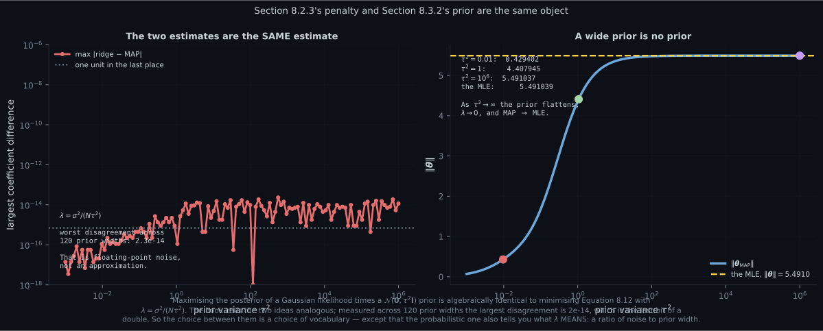
Reading the plot

The first figure is the chapter’s central claim, and it is a claim about an identity rather than an analogy. The left panel plots the largest coefficient disagreement between ridge regression and MAP across $120$ prior widths spanning six orders of magnitude. The curve never rises above $1.24\times10^{-14}$, and the dotted reference line is one unit in the last place of a double at this scale. There is no regime where they differ.

That is stronger than the book’s “analogous”, and it is worth being precise about why it holds: the log of a Gaussian prior is a negative quadratic in $\boldsymbol\theta$, and $-\log$ of it is $\lVert\boldsymbol\theta\rVert^2/(2\tau^2)$ plus a constant. A squared-norm penalty is a log-Gaussian prior. Any other prior gives a different penalty — a Laplace prior gives the $\ell_1$ penalty of lasso — so the correspondence is general even though this instance is specific.

The right panel shows the limit behaviour. As $\tau^2$ grows the prior flattens, $\lambda \to 0$, and $\lVert\boldsymbol\theta\rVert$ climbs to $5.491037$ against an MLE value of $5.491039$. A vague prior is no prior, exactly as it should be.

And here is what the probabilistic vocabulary adds, given the answers are identical. In §8.2.3, $\lambda$ is a dimensionless knob with no meaning, tuned by cross-validation. Here it is $\sigma^2/(N\tau^2)$ — which immediately predicts three things you would otherwise have to discover empirically: noisier data should be shrunk harder, a more confident prior should shrink harder, and more data should shrink less. Same number, more information about where to look for it.

The second figure is where I had to correct my reading of the book. Figure 8.6’s caption says the prior “biases the slope to be less steep and the intercept to be closer to zero”. I expected both coefficients to shrink monotonically. The intercept does — from $8.8074$ steadily toward zero. The slope does not. It rises from $2.1225$ to a peak of $2.2988$ at $\tau^2 = 31.71$, and only falls below the MLE once $\tau^2 < 1$.

The mechanism is worth understanding because it generalises. The prior penalises $\lVert\boldsymbol\theta\rVert^2 = \theta_0^2 + \theta_1^2$, not each coefficient. The intercept is cheap to shrink — the data barely constrains it, because age ranges from $26$ to $68$ and the intercept lives at $0$, far outside. But the line still has to pass near a data cloud centred at age $42$ and salary $98$. Pull the $y$-intercept toward zero and the only way to still reach that cloud is a steeper slope. The two coefficients trade.

So the book’s statement is correct about the destination and not about the path. And the practical consequence is page 801’s advice from the other direction: centre your inputs and exclude the intercept from the penalty, or the regulariser will spend its budget on the coefficient that means the least.

The third figure turns Figure 8.8’s three words into three numbers, and the surprise is in the training-risk column. Overfitting achieves $0.005232$ — the lowest training risk of the three, $22\times$ better than the model that actually generalises. Its expected risk is $3.9173$, giving a ratio of $748.8$. Underfitting sits at $0.477771$ and $0.7254$, a ratio of only $1.5$.

The asymmetry is the practical lesson. Underfitting announces itself: a training risk of $0.478$ from a two-parameter model is visibly bad, and you can see it without any held-out data. Overfitting is silent — every training-side number is excellent, and the parameter norm of $3616.98$ is the only clue available without a test set. That is precisely why the book’s margin note recommends comparing training and test risk during cross-validation, and why page 802’s parameter-norm measurement matters: it is the one warning sign you can read off the training fit alone.

From the book

This page covers §8.3.2, §8.3.3 and §8.3.4 of Mathematics for Machine Learning by Deisenroth, Faisal and Ong (draft of 2019-12-11). Equation 8.19 is Bayes’ theorem for parameters and 8.20 the proportionality that drops $p(\mathbf{x})$; the terms posterior, prior and likelihood and the remark that $p(\mathbf{x})$ “may be difficult to estimate” are the book’s. Example 8.6 assumes a zero-mean Gaussian prior and notes the conjugacy of §6.6.1, deferring details to Chapter 9. Figure 8.6 compares the MLE and MAP predictions at $x = 60$ and states that the prior biases the slope and intercept. The characterisation of MAP as bridging the non-probabilistic and probabilistic worlds “but it still only produces a point estimate” is verbatim. Figure 8.7 is the model-class picture with $M_{\boldsymbol\theta}$, $M^*$ and $M_{\boldsymbol\theta_0}$; Figure 8.8 and §8.3.3 give the three cases, the characterisations of over- and underfitting, the observation that an overly flexible class “will find some useful signal in the noise itself”, and the margin note about detecting overfitting via low training risk beside high test risk. §8.3.4 supplies Equation 8.21 and the generalized linear model pointer to McCullagh and Nelder (1989). The exact correspondence $\lambda = \sigma^2/(N\tau^2)$ measured to $1.24\times10^{-14}$, the non-monotone slope peaking at $2.2988$, the risks attached to Figure 8.8’s three cases, and the closed form $\hat\theta_{\text{MAP}} = N\bar{y}/(N + \sigma^2/\tau^2)$ are this module’s additions.

Pitfalls

Thinking a prior and a penalty are merely analogous

Measured across $120$ prior widths spanning six orders of magnitude, the largest disagreement between ridge and MAP is $1.24\times10^{-14}$. They are one estimator with two names. The consequence is practical: if you tune $\lambda$ by cross-validation you have implicitly chosen $\sigma^2/(N\tau^2)$, and that ratio is a statement about how noisy you think your data is relative to how confident you are.

Expecting an isotropic prior to shrink every coefficient

It shrinks $\lVert\boldsymbol\theta\rVert$, which is a different thing. Measured on Table 8.2: as the prior tightens the intercept falls monotonically from $8.8074$ while the slope rises from $2.1225$ to $2.2988$ before eventually falling. Coefficients trade against each other, and the one the data constrains least gets shrunk first.

Regularising an uncentred intercept

This is the practical form of the previous pitfall. The intercept sits at $x = 0$, usually far outside the data, so the likelihood barely constrains it and the prior shrinks it almost for free — forcing the other coefficients to compensate. Centre the inputs and exclude $\theta_0$ from the penalty. Equation 8.4’s unit-feature trick makes this easy to forget, since $\theta_0$ looks like any other coefficient.

Treating MAP as Bayesian inference

MAP writes down a posterior and then keeps only the location of its peak. The book is explicit that it “still only produces a point estimate of the parameters”. Everything about the posterior’s width — which is the part that would let you say how confident the prediction is — is discarded. §8.4 keeps it.

Reading a low training risk as a good fit

Measured on Figure 8.8’s three cases: the overfitting model has the lowest training risk of the three, $0.005232$ against the good model’s $0.113967$, and an expected risk $748.8\times$ its training figure. Underfitting is visible from the training data alone; overfitting is not. The only training-side warning is the parameter norm — $3616.98$ against $5.67$.

Assuming a Gaussian prior is the only option

It is the one that produces a squared-norm penalty, because $-\log$ of a Gaussian is a quadratic. A Laplace prior gives $\lVert\boldsymbol\theta\rVert_1$ and hence lasso, with entirely different behaviour — it sets coefficients to exactly zero. The correspondence “prior equals penalty” is general; the correspondence “Gaussian prior equals ridge” is the specific instance.

Compare

	MLE, §8.3.1	MAP, §8.3.2	Bayesian inference, §8.4
what it maximises	the likelihood	the posterior	nothing — it integrates
needs a prior	no	yes	yes
needs $p(\mathbf{x})$	no	no, it cancels	yes
what it returns	a point	a point	a distribution
overfits on small data	yes	less	no, it averages
equivalent in §8.2	plain ERM	ERM with a penalty	no equivalent
computational problem	optimisation	optimisation	integration

prior on $\boldsymbol\theta$	the penalty it implies	behaviour
$\mathcal{N}(\mathbf{0}, \tau^2\mathbf{I})$	$\lambda\lVert\boldsymbol\theta\rVert^2$, ridge	shrinks all coefficients smoothly
Laplace	$\lambda\lVert\boldsymbol\theta\rVert_1$, lasso	sets some to exactly zero
uniform (improper)	none	recovers the MLE
$\mathcal{N}(\mathbf{m}, \tau^2\mathbf{I})$	$\lambda\lVert\boldsymbol\theta - \mathbf{m}\rVert^2$	shrinks toward $\mathbf{m}$, not the origin

pch.quizTag Do you know what the prior is doing?

1. A zero-mean Gaussian prior of variance tau squared on theta gives exactly ridge regression. With what lambda?

   A lambda = tau squared B lambda = sigma squared over (N tau squared) C lambda = 1 over tau squared D There is no exact correspondence, only an analogy
   pch.quizShowAnswer

   B — lambda = sigma squared over (N tau squared) — Measured across 120 prior widths, the largest disagreement is 1.24e-14 — floating point noise. And the formula tells you what lambda MEANS: a ratio of noise variance to prior variance, divided by the sample size. So noisier data shrinks harder, a tighter prior shrinks harder, and more data shrinks less.

2. The book says a zero-mean prior biases the slope to be less steep. Measured on Table 8.2, what actually happens as the prior tightens?

   A Both coefficients shrink monotonically, as stated B The intercept shrinks monotonically but the slope first RISES, peaking at 2.2988 against an MLE slope of 2.1225 C Neither coefficient changes D The slope shrinks and the intercept grows
   pch.quizShowAnswer

   B — The intercept shrinks monotonically but the slope first RISES, peaking at 2.2988 against an MLE slope of 2.1225 — An isotropic prior penalises the NORM, not each entry. The intercept is cheap to shrink because the data barely constrains it — but pulling the y-intercept toward zero while the line must still reach a data cloud centred at age 42 forces a steeper slope. The claim is right about the destination and wrong about the path.

3. Why can MAP estimation ignore p(x), the denominator of Bayes' theorem?

   A Because it is always equal to one B Because it does not depend on theta, so it cannot affect which theta maximises the posterior C Because it is assumed Gaussian D It cannot be ignored; MAP requires computing it
   pch.quizShowAnswer

   B — Because it does not depend on theta, so it cannot affect which theta maximises the posterior — It is a constant with respect to the maximisation. The book notes this hides a density that 'may be difficult to estimate' — it is an integral over all of parameter space. Section 8.4 needs it and Section 8.3.2 does not, which is a large part of why MAP is so much cheaper than full Bayesian inference.

4. In Figure 8.8's three cases, which model has the lowest training risk?

   A The one that fits well, at 0.113967 B The overfitting one, at 0.005232 — 22 times lower than the model that actually generalises C The underfitting one D They are all approximately equal
   pch.quizShowAnswer

   B — The overfitting one, at 0.005232 — 22 times lower than the model that actually generalises — And its expected risk is 3.9173, a ratio of 748.8. That asymmetry is the practical lesson: underfitting is visible from training data alone, since a training risk of 0.478 from two parameters is obviously bad, while overfitting produces excellent training numbers. The only training-side clue is the parameter norm — 3616.98 against 5.67.

5. What does MAP estimation still not give you?

   A A way to incorporate prior knowledge B Anything about the posterior beyond the location of its peak — it is still a point estimate C A regularised solution D Protection against overfitting
   pch.quizShowAnswer

   B — Anything about the posterior beyond the location of its peak — it is still a point estimate — The book's phrasing is that MAP bridges the two worlds because it acknowledges the need for a prior 'but it still only produces a point estimate of the parameters'. You write down a whole distribution and keep one number from it. The width — the part that would tell you how confident to be — is discarded, and Section 8.4 is what happens when you keep it.

🧪 Try It Yourself

Exercise 1 – A prior is a penalty

pch.exerciseTag pch.exerciseTitle

Exercise 2 – The closed form for a Gaussian mean

pch.exerciseTag pch.exerciseTitle

Exercise 3 – The slope does not shrink monotonically

pch.exerciseTag pch.exerciseTitle

Exercise 4 – Figure 8.8’s three cases

pch.exerciseTag pch.exerciseTitle

Exercise 5 – A vague prior is no prior

pch.exerciseTag pch.exerciseTitle

Recall card

• Equation 8.19 is Bayes’ theorem for parameters, and Equation 8.20 drops the denominator because p(x) does not depend on theta. That denominator is an integral over all of parameter space, and Section 8.4 will need it.
• MAP minimises the negative log-POSTERIOR instead of the negative log-likelihood — one extra term, from the prior.
• A zero-mean Gaussian prior of variance tau squared IS the ridge penalty, with lambda = sigma squared over (N tau squared). Measured across 120 prior widths spanning six orders of magnitude, the worst disagreement is 1.24e-14.
• What the probabilistic vocabulary buys, given the answers match: it tells you what lambda MEANS. Noisier data shrinks harder, a tighter prior shrinks harder, more data shrinks less — all read straight off the formula.
• The correspondence is general, the instance is specific. Minus the log of a Gaussian is a quadratic, hence the squared norm. A Laplace prior gives the L1 penalty of lasso, which sets coefficients to exactly zero.
• An isotropic prior shrinks the NORM, not each coefficient. Measured on Table 8.2: the intercept falls monotonically from 8.8074 while the slope RISES from 2.1225 to a peak of 2.2988 at tau squared = 31.71. Coefficients trade, and the one the data constrains least gets shrunk first.
• So centre your inputs and exclude the intercept from the penalty. The intercept lives at x = 0, usually far outside the data, so it is cheap to shrink and shrinking it forces the others to compensate.
• Closed form for a Gaussian mean: theta-MAP is the sample mean times N over (N + sigma squared over tau squared) — which equals 1/(1+lambda), the same expression page 803 derived from the penalty side with no probability in sight.
• MAP is still a point estimate. The book’s phrasing: it bridges the two worlds because it acknowledges the prior, “but it still only produces a point estimate”. You write down a posterior and keep its peak.
• Section 8.3.3’s three cases, measured on 14 points: overfitting (degree 11) has training risk 0.005232, expected risk 3.9173, ratio 748.8, norm 3616.98. Underfitting (degree 1) has 0.477771 and 0.7254. Fitting well (degree 4) has 0.113967 and 0.3806.
• Overfitting has the LOWEST training risk of the three — 22 times lower than the good model. Underfitting is visible from training data alone; overfitting is not, and the parameter norm is the only training-side warning.
• Section 8.3.4: putting a nonlinear function on a linear predictor, p(y | x, theta) = phi(theta-transpose x), gives the generalized linear model — binary classification, count data, and the exponential family of Section 6.6.

Next: stop throwing the posterior away. Probabilistic Modeling and Inference