What you’ll learn

• why a 0.9642 held-out score is not evidence that a model works
• the accuracy-versus-transparency trade-off, measured: a 0.0651 accuracy spread against a 1,803× spread in how much you have to read
• the difference between global and local explanations, and why one does not give you the other
• the four questions interpretability actually answers, and which tool answers each
• what “the model is 0.96 accurate” leaves out, and how a single permutation catches it
• where interpretability is a legal requirement rather than a nice-to-have

A model that was right for the wrong reason

Two hospitals, one disease, one dataset each. Both datasets contain the same honest clinical markermarker, and both contain scanner_idscanner_id — which machine took the image. At the training hospital, the sick were almost all scanned on machine 1, purely because of how the wards were laid out. The correlation between scanner_idscanner_id and the diagnosis there is 0.9460.

At the second hospital, scanners were assigned as patients arrived. Correlation: −0.0007.

Train a random forest on the first hospital’s data and hold out 30% of it:

full = RandomForestClassifier(n_estimators=300, min_samples_leaf=50,
                              random_state=0).fit(X_train, y_train)
 
print(f"{full.score(X_holdout, y_holdout):.4f}")   # 0.9642

full = RandomForestClassifier(n_estimators=300, min_samples_leaf=50,
                              random_state=0).fit(X_train, y_train)
 
print(f"{full.score(X_holdout, y_holdout):.4f}")   # 0.9642

0.9642. A clean train/test split, no leakage across the split, no tuning on the test set. Every methodological rule in Phase 02 was followed. This model ships.

Now run it at the second hospital.

figure0.9642 at home, 0.4998 next doormatplotlib

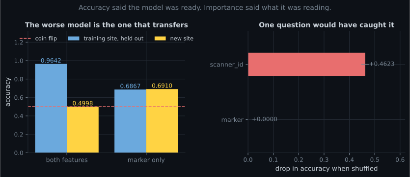
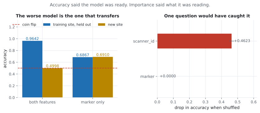
0.4998. Not degraded — worthless. And the model that looked worse, the one trained on markermarker alone, went from 0.6867 to 0.6910: unchanged, because it learned something true.

Nothing about accuracy could have warned you. The held-out score was honest about what it measured; it just measured a world where the shortcut held. Only a question about mechanism separates the two models before deployment, and interpretability is the vocabulary for asking it:

from sklearn.inspection import permutation_importance
 
pi = permutation_importance(full, X_holdout, y_holdout, n_repeats=30, random_state=0)
for name, mean, sd in zip(X.columns, pi.importances_mean, pi.importances_std):
    print(f"{name:12s} {mean:+.4f} +- {sd:.4f}")
 
# marker       +0.0000 +- 0.0000
# scanner_id   +0.4623 +- 0.0155

from sklearn.inspection import permutation_importance
 
pi = permutation_importance(full, X_holdout, y_holdout, n_repeats=30, random_state=0)
for name, mean, sd in zip(X.columns, pi.importances_mean, pi.importances_std):
    print(f"{name:12s} {mean:+.4f} +- {sd:.4f}")
 
# marker       +0.0000 +- 0.0000
# scanner_id   +0.4623 +- 0.0155

markermarker contributes +0.0000, to four decimal places, with a standard deviation of 0.0000 across 30 shuffles. The clinical signal is not being used at all. Every point of accuracy above chance comes from the scanner ID. That is a sentence you can take to a domain expert, and any radiologist would have stopped the deployment on the spot.

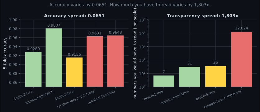
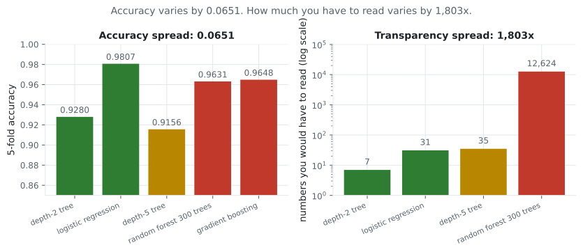
The trade-off is real, and much smaller than its reputation

The standard defence of black boxes is that transparency costs accuracy. Measure it. Five models on the Wisconsin breast-cancer data, 5-fold cross-validation, and alongside each one the count of numbers a human would have to read to know exactly what it does — coefficients for the linear model, nodes across the whole ensemble for the forest:

figureAccuracy varies by 0.0651. How much you have to read varies by 1,803x.matplotlib

The whole accuracy range is 0.0651, and the most accurate model here is the fully transparent one. Reading effort ranges over 1,803×.

This is one dataset, and it is deliberately favourable to linear models — thirty engineered, well-scaled features and a nearly linearly separable target. On high-dimensional unstructured data (images, audio, text) the gap is genuine and large. The honest summary is:

• On tabular data of modest size, always fit the transparent baseline first. It frequently wins, and when it loses it usually loses by less than the effort of explaining the winner costs you.
• When the black box does win by a margin that matters, you have not bought an excuse to skip interpretability. You have bought an obligation to add it, because the model is now the only place that knowledge lives.

Global and local are different questions

figureTwo questions interpretability answersmatplotlib

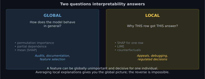
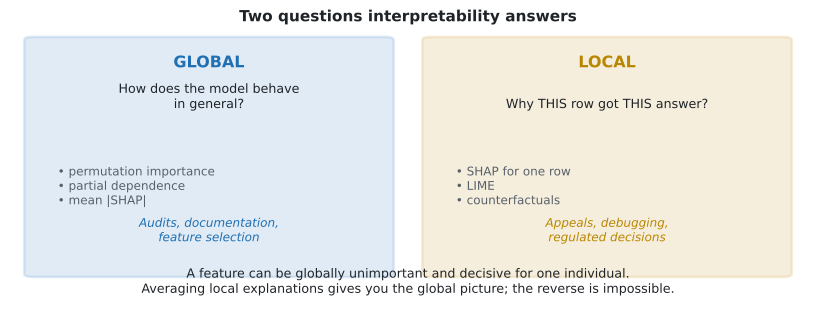
The asymmetry is worth stating precisely, because it is the reason the following pages exist in the order they do. Let $\phi_j^{(i)}$ be feature $j$’s contribution to row $i$. Global importance is an average over rows:

The map from the collection $\{\phi_j^{(i)}\}$ to $I_j$ throws information away and cannot be inverted. Concretely, on the four-feature linear model used throughout this phase — true coefficients $3, -2, 1, 0$ — the global picture is unambiguous:

f2_weakf2_weak is third by a wide margin globally. It is nevertheless the decisive feature on 43 rows — more than one in ten. Row 102 is one of them:

x    = [ 0.0367  0.2920 -2.5791  0.5549]
phi  = [+0.2500 -0.5400 -2.5453 +0.0051]
base = -0.2102     prediction = -3.0404

x    = [ 0.0367  0.2920 -2.5791  0.5549]
phi  = [+0.2500 -0.5400 -2.5453 +0.0051]
base = -0.2102     prediction = -3.0404

The prediction is $-3.0404$ and the third feature accounts for $-2.5453$ of the $-2.8302$ move away from the base value. If this were a declined loan, the applicant’s answer is f2_weakf2_weak — the feature the global report calls minor. Show them the global chart and you have told them something true about the model and false about their case.

And f3_uselessf3_useless, whose true coefficient is exactly zero, is the largest contribution on 0 of 400 rows. Genuine irrelevance survives both views.

Which tool for which question

  flowchart TD
  Q{"What are you actually asking?"}
  Q -->|"Which features drive the model overall?"| G["Permutation importance
on HELD-OUT data"]
  Q -->|"Which direction does this feature push?"| P["Partial dependence
+ ICE curves"]
  Q -->|"Why did THIS row get THIS answer?"| S["SHAP for one row
sums exactly to the prediction"]
  Q -->|"What would have to change to flip it?"| C["Counterfactual
nearest row with the other label"]
  Q -->|"Is the model treating groups differently?"| F["Group metrics
at a fixed threshold"]
  G --> W{"Is the answer defensible
to a domain expert?"}
  P --> W
  S --> W
  C --> W
  F --> W
  W -->|"no"| X["Do not deploy.
The model found a shortcut."]
  W -->|"yes"| D["Deploy, and keep
measuring in production"]

Every arrow out of that first node is a different computation, and picking the wrong one produces a confident answer to a question nobody asked. The most common mismatch in practice: reaching for global importance when the question was about one person.

Where it stops being optional

Three situations turn interpretability from good engineering into a requirement.

Contestable decisions. Credit, hiring, insurance, benefits, admissions. Under the EU’s GDPR (Article 22 and the surrounding recitals) a person subject to a significant automated decision has rights of contestation, which in practice requires the deciding organisation to be able to say something specific about the individual decision. Whatever the precise legal reading — and it is still argued — a per-row explanation is the only artefact that answers “why me”. That is a local requirement, so mean importance does not satisfy it.

Safety-critical and clinical settings. A model that recommends a treatment is used by someone who must be able to override it. An override requires a reason, and a reason requires knowing what the model looked at. The scanner-ID failure above is the canonical example, and it is not hypothetical: shortcut learning from acquisition artefacts is a recurring finding in medical imaging.

Anything you will have to debug. This one applies to every model you will ever build. When accuracy falls in production, “which features is it leaning on now, compared with training?” is the first useful question. If you cannot answer it, your only remaining move is to retrain and hope — see Monitoring Model Drift.

See it move

The shortcut model does not fail because the world changed a lot. It fails because one correlation weakened. Consider the crudest possible shortcut model — the rule “predict sick if scanner_idscanner_id is 1” — and an honest model that thresholds markermarker at 0.5. Both accuracies are exactly computable.

If the deployment site’s leak strength is $\ell$ (the fraction of patients whose scanner matches their diagnosis, the rest assigned at random), the shortcut rule is correct with probability

while the honest rule sits at $\Phi(0.5) \approx 0.6915$ regardless, because it reads a signal that travels. Drag to move the new site’s leak strength and watch the crossover.

Two things are worth noticing. The shortcut’s accuracy is a straight line in $\ell$ — a property of the site, not of the model — and at the training site’s $\ell = 0.95$ it reads 0.9750, comfortably above the honest rule’s 0.6915. Any selection procedure that compares held-out scores at one site will pick the shortcut every time. And at $\ell = 0$ the shortcut is not merely worse, it is at 0.5000, which is what “no information” looks like.

In code: the four-line audit

Before any model goes anywhere, run this. It is cheap and it has caught real bugs.

"""The smallest interpretability check worth running on every model."""
 
import numpy as np
from sklearn.inspection import permutation_importance
 
 
def audit(model, X_holdout, y_holdout, expectations=None, n_repeats=30):
    """Print what the model leans on, and flag anything the domain did not expect.
 
    `expectations` is a set of column names a domain expert said should matter.
    Anything important that is NOT in that set is the interesting output.
    """
    pi = permutation_importance(model, X_holdout, y_holdout,
                                n_repeats=n_repeats, random_state=0)
    order = np.argsort(pi.importances_mean)[::-1]
    total = pi.importances_mean[pi.importances_mean > 0].sum()
 
    print(f"{'feature':22s} {'importance':>12s} {'sd':>8s} {'share':>7s}")
    for i in order:
        name = X_holdout.columns[i]
        mean, sd = pi.importances_mean[i], pi.importances_std[i]
        share = mean / total if total > 0 and mean > 0 else 0.0
        flag = ""
        if expectations is not None and name not in expectations and share > 0.10:
            flag = "  <-- NOT EXPECTED TO MATTER"
        if mean < -2 * sd:
            flag = "  <-- ACTIVELY MISLEADING"
        print(f"{name:22s} {mean:+12.4f} {sd:8.4f} {share:6.1%}{flag}")
 
 
audit(full, X_holdout, y_holdout, expectations={"marker"})
# feature                  importance       sd   share
# scanner_id                  +0.4623   0.0155 100.0%  <-- NOT EXPECTED TO MATTER
# marker                      +0.0000   0.0000   0.0%

"""The smallest interpretability check worth running on every model."""
 
import numpy as np
from sklearn.inspection import permutation_importance
 
 
def audit(model, X_holdout, y_holdout, expectations=None, n_repeats=30):
    """Print what the model leans on, and flag anything the domain did not expect.
 
    `expectations` is a set of column names a domain expert said should matter.
    Anything important that is NOT in that set is the interesting output.
    """
    pi = permutation_importance(model, X_holdout, y_holdout,
                                n_repeats=n_repeats, random_state=0)
    order = np.argsort(pi.importances_mean)[::-1]
    total = pi.importances_mean[pi.importances_mean > 0].sum()
 
    print(f"{'feature':22s} {'importance':>12s} {'sd':>8s} {'share':>7s}")
    for i in order:
        name = X_holdout.columns[i]
        mean, sd = pi.importances_mean[i], pi.importances_std[i]
        share = mean / total if total > 0 and mean > 0 else 0.0
        flag = ""
        if expectations is not None and name not in expectations and share > 0.10:
            flag = "  <-- NOT EXPECTED TO MATTER"
        if mean < -2 * sd:
            flag = "  <-- ACTIVELY MISLEADING"
        print(f"{name:22s} {mean:+12.4f} {sd:8.4f} {share:6.1%}{flag}")
 
 
audit(full, X_holdout, y_holdout, expectations={"marker"})
# feature                  importance       sd   share
# scanner_id                  +0.4623   0.0155 100.0%  <-- NOT EXPECTED TO MATTER
# marker                      +0.0000   0.0000   0.0%

The expectationsexpectations argument is the part people skip, and it is the part that does the work. A ranked list of importances is data; a ranked list checked against what a domain expert expected is a finding. On the shortcut model it prints in one line what a month in production would have taught you the expensive way.

Pitfalls

Recap

• A forest scored 0.9642 on a clean held-out split and 0.4998 at the next site, because it read scanner_idscanner_id (correlation 0.9460 there, −0.0007 elsewhere) rather than the patient.
• The model that scored 0.6867 without the shortcut held up at 0.6910. The worse model transferred.
• Permutation importance on the training site’s own held-out data already said so: scanner_idscanner_id +0.4623, markermarker +0.0000 ± 0.0000.
• Measured on the breast-cancer data, accuracy spans 0.0651 across five models while reading effort spans 1,803× — and the most accurate model is the transparent one, at 0.9807.
• Global and local are different questions. f2_weakf2_weak is third globally (mean $|\phi|$ 0.8013) and decisive on 43 of 400 rows.
• Averaging local explanations gives the global picture. The reverse is impossible.

🧪 Try It Yourself

Exercise 1 – Measure the trade-off instead of assuming it

Exercise 2 – Build a shortcut and watch it die

Exercise 3 – Ask the model what it read

Exercise 4 – Delete the shortcut, keep the model

Exercise 5 – Show that global importance cannot answer a local question

Exercise 6 – Build the shortcut, then catch it

Next

Feature Importance and Its Traps — permutation importance caught the shortcut on this page. The next page shows the three ways the same tool lies to you, starting with a column of pure noise that took 38.53% of the credit.