What you’ll learn

• the Shapley value from its definition, implemented in about fifteen lines
• the additivity guarantee, verified to an error of 0.00e+00
• the four axioms that make Shapley values the only attribution with these properties
• mean $|\mathrm{SHAP}|$ as global importance, and how well it recovers known coefficients
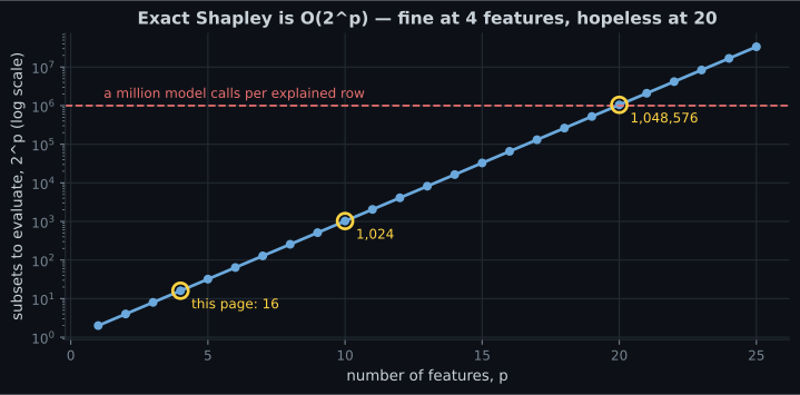
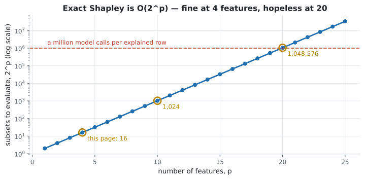
• why exact computation is $O(2^p)$ — 16 subsets at 4 features, a million at 20
• what SHAP does not tell you

No shapshap library on this page. Everything here is computed exactly, from the definition, with numpy and scikit-learn — which is both reproducible and considerably more informative than a library call.

The question SHAP answers

Importance and PDP are global: they describe the model’s behaviour across a dataset. Neither answers the question a customer, a regulator or an on-call engineer actually asks:

This specific prediction came out at 0.83. Why?

The natural framing is a budget. The model predicted $\hat{f}(x)$ for this row. If you knew nothing about the row, you would predict the average, $\mathbb{E}[\hat{f}]$. The difference between those two numbers has to be divided up among the features, and each feature’s share is its contribution.

That is an allocation problem, and allocation problems have a canonical answer from cooperative game theory.

The Shapley value

Treat the features as players in a game whose payoff is the model’s output. The value of a coalition $S$ is what the model predicts when only the features in $S$ are known:

The features not in $S$ are set to their background values — typically the dataset mean.

A feature’s marginal contribution to a coalition is what it adds when it joins: $v(S \cup \{j\}) - v(S)$. That depends on which coalition it joins, so the Shapley value averages over all of them, weighted by the Shapley kernel:

The weight has a clean interpretation: it is the probability that, in a uniformly random ordering of all $p$ features, exactly the members of $S$ arrive before $j$. So $\phi_j$ is the average marginal contribution of feature $j$ over every possible ordering of the features.

In fifteen lines

import itertools
import math
 
import numpy as np
 
 
def exact_shapley(predict, x, background):
    """Exact Shapley values, straight from the definition. O(2^p)."""
    p = len(x)
    phi = np.zeros(p)
 
    def value(subset):
        """v(S): known features from x, unknown ones from the background."""
        z = background.copy()
        for j in subset:
            z[j] = x[j]
        return float(predict(z.reshape(1, -1))[0])
 
    for j in range(p):
        rest = [k for k in range(p) if k != j]
        for size in range(len(rest) + 1):
            weight = (math.factorial(size) * math.factorial(p - size - 1)
                      / math.factorial(p))
            for subset in itertools.combinations(rest, size):
                phi[j] += weight * (value(list(subset) + [j]) - value(list(subset)))
    return phi

import itertools
import math
 
import numpy as np
 
 
def exact_shapley(predict, x, background):
    """Exact Shapley values, straight from the definition. O(2^p)."""
    p = len(x)
    phi = np.zeros(p)
 
    def value(subset):
        """v(S): known features from x, unknown ones from the background."""
        z = background.copy()
        for j in subset:
            z[j] = x[j]
        return float(predict(z.reshape(1, -1))[0])
 
    for j in range(p):
        rest = [k for k in range(p) if k != j]
        for size in range(len(rest) + 1):
            weight = (math.factorial(size) * math.factorial(p - size - 1)
                      / math.factorial(p))
            for subset in itertools.combinations(rest, size):
                phi[j] += weight * (value(list(subset) + [j]) - value(list(subset)))
    return phi

That is the whole algorithm. Everything the shapshap library does beyond this is either an approximation to make it fast or a plotting convenience.

See it move

The kernel weight is easier to believe as orderings than as factorials. Take a model small enough to write down completely — three binary features, background all zeros, explaining $x = (1,1,1)$:

The $3x_1x_3$ term means $x_3$ is worth nothing on its own and worth 3 once $x_1$ has arrived, so the order genuinely matters. Enumerating all eight coalitions gives the value function, and the exact Shapley values work out to $\phi_1 = 3.5$, $\phi_2 = 1.0$, $\phi_3 = 1.5$ — summing to $f(1,1,1) = 6$, as efficiency requires.

The sketch below draws one random ordering at a time, adds each feature in turn, and credits it with whatever the prediction moved. The running average is the Shapley value.

Two invariants are worth watching. Every ordering’s credits sum to 6, because the walk always starts at $v(\emptyset)$ and ends at $f(x)$ — that is efficiency, holding per ordering, not just on average. And $x_3$’s credit is 0 when it arrives before $x_1$ and 3 when it arrives after, which averages to 1.5. Nothing about the Shapley value is mysterious once you see it as bookkeeping over arrival orders; the only hard part is that there are $p!$ of them.

Additivity, verified

The defining property — the one that makes SHAP usable in a regulated setting — is local accuracy, also called efficiency:

The contributions do not merely indicate direction. They sum exactly to the gap between the prediction and the base value. Here it is on a linear model whose true coefficients are $3, -2, 1, 0$, explaining row 0:

figurebase −0.2102 + contributions +1.3965 = +1.1863, error 0.00e+00matplotlib

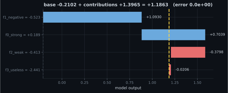
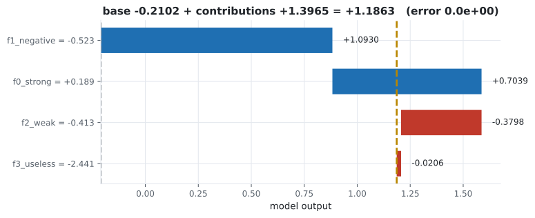
Note f1_negativef1_negative. Its coefficient is −2.0, and its SHAP value is +1.0930 — positive. There is no contradiction: the feature’s value is −0.523, which is below the background mean, so a negative coefficient times a below-average value pushes the prediction up. SHAP attributes the effect of this row’s value, not the coefficient.

That distinction is the most common misreading of a SHAP plot.

The four axioms

Shapley values are not one reasonable attribution among many. They are the unique allocation satisfying all four of:

The uniqueness result is Shapley’s 1953 theorem. It is why SHAP has displaced ad-hoc attribution methods: any method violating one of those axioms can be shown to produce an indefensible answer on some input.

The dummy axiom is visible above: f3_uselessf3_useless has a true coefficient of 0 and a fitted coefficient of 0.0086, and its SHAP value is −0.0206 — not exactly zero, because the fitted coefficient is not exactly zero, but two orders of magnitude below the others.

Global importance from local explanations

Average the absolute SHAP values across many rows and you get a global importance measure — one built up from per-row attributions rather than imposed from above:

Over 120 rows, against the coefficients that actually generated the data:

figureExact Shapley values on a model whose coefficients are 3, −2, 1 and 0matplotlib

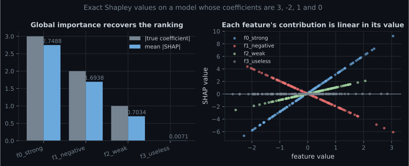
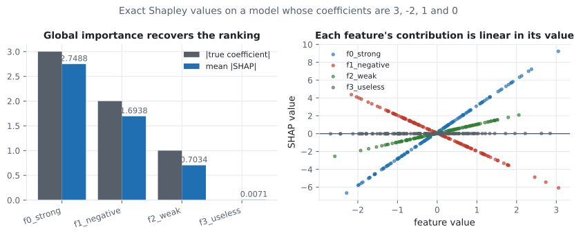
Note that mean $|\mathrm{SHAP}|$ is not equal to the coefficient. For a linear model $\phi_j = \beta_j (x_j - \bar{x}_j)$, so the mean absolute value is

With standard normal features that expectation is $\sqrt{2/\pi} \approx 0.798$, and indeed $3.0 \times 0.798 = 2.394$ — close to, though not exactly, the 2.7488 measured, because the fitted coefficient is 2.9798 and the sample is finite.

The ranking is what transfers. The magnitudes are in units of model output, not of the features.

The cost

Exact computation evaluates $2^{p}$ subsets per feature. That is fine here and hopeless in practice.

figureExact Shapley is O(2^p) — fine at 4 features, hopeless at 20matplotlib

Hence the approximations, all of which are in the shapshap library:

TreeSHAP is exact and fast, which is why SHAP became standard on tabular data specifically. For gradient boosting and random forests you get the exact Shapley values in polynomial time.

# In production, on a tree model:
import shap
explainer = shap.TreeExplainer(model)
shap_values = explainer(X)          # exact, and fast

# In production, on a tree model:
import shap
explainer = shap.TreeExplainer(model)
shap_values = explainer(X)          # exact, and fast

Choosing an explainer

  flowchart TD
  A["Model you need to explain"] --> B{"What kind?"}
  B -->|"tree ensemble --
RF, GBM, XGBoost, LightGBM"| T["TreeExplainer.
Exact, polynomial time.
No sampling error to report."]
  B -->|"linear or logistic"| L["LinearExplainer.
Closed form: beta_j times
(x_j minus its mean)."]
  B -->|"neural network"| D["DeepExplainer or
GradientExplainer."]
  B -->|"anything else --
SVM, kNN, a pipeline,
a remote API"| K["KernelExplainer.
Model-agnostic and slow."]
  K --> K2{"How many rows to explain?"}
  K2 -->|"a handful"| K3["Fine as is."]
  K2 -->|"thousands"| K4["Summarise the background
with shap.kmeans, cap nsamples,
and report the sampling error."]
  T --> V{"Interpreting the output"}
  L --> V
  D --> V
  K3 --> V
  K4 --> V
  V --> V1["Check additivity:
base value + sum of phi
= the model's prediction."]
  V1 --> V2["Remember what it is NOT:
attribution to the model,
not a causal effect."]

The branch to be honest about is KernelExplainerKernelExplainer. It is the only one that works on anything, and it is approximate, background-dependent and expensive — three properties that must appear in whatever you write down next to the numbers. A SHAP plot with no statement of which explainer produced it is an unlabelled measurement.

What SHAP does not tell you

Four limits, all of which get violated in practice.

It is not causal. $\phi_j$ says the model’s output would differ if this feature were at its background value. It says nothing about what happens if you change the feature in the world. “Increase income by 10k to get approved” is not something a SHAP value licenses.

The background distribution is a choice, and it changes the answer. The base value is $v(\emptyset)$, computed from whatever background you supply. Explain a loan rejection against all applicants and you get one story; against rejected applicants only you get another. Both are valid; they answer different questions. State which you used.

Correlated features share credit arbitrarily. With two near-duplicate columns, the marginal contribution of each depends on whether the other is already in the coalition, and the Shapley average splits the credit between them — the same split-credit problem as permutation importance. Group correlated features before explaining.

It explains the model, not the truth. If the model learned a spurious pattern, SHAP will faithfully report that spurious pattern as the reason. A confident, well-formed explanation of a wrong prediction is still wrong.

In code

import numpy as np
from sklearn.linear_model import LinearRegression
 
rng = np.random.default_rng(2)
n, coefs = 800, np.array([3.0, -2.0, 1.0, 0.0])
X = rng.normal(0, 1, (n, len(coefs)))
y = X @ coefs + rng.normal(0, 0.3, n)
 
model = LinearRegression().fit(X, y)
background = X.mean(axis=0)
 
phi = exact_shapley(model.predict, X[0], background)
base = float(model.predict(background.reshape(1, -1))[0])
pred = float(model.predict(X[0].reshape(1, -1))[0])
 
print("contributions", np.round(phi, 4))
# [ 0.7039  1.093  -0.3798 -0.0206]
print(f"base {base:+.4f} + sum {phi.sum():+.4f} = {base + phi.sum():+.4f}")
print(f"actual prediction                     = {pred:+.4f}")
print(f"additivity error                      = {abs(base + phi.sum() - pred):.2e}")
# additivity error                      = 0.00e+00

import numpy as np
from sklearn.linear_model import LinearRegression
 
rng = np.random.default_rng(2)
n, coefs = 800, np.array([3.0, -2.0, 1.0, 0.0])
X = rng.normal(0, 1, (n, len(coefs)))
y = X @ coefs + rng.normal(0, 0.3, n)
 
model = LinearRegression().fit(X, y)
background = X.mean(axis=0)
 
phi = exact_shapley(model.predict, X[0], background)
base = float(model.predict(background.reshape(1, -1))[0])
pred = float(model.predict(X[0].reshape(1, -1))[0])
 
print("contributions", np.round(phi, 4))
# [ 0.7039  1.093  -0.3798 -0.0206]
print(f"base {base:+.4f} + sum {phi.sum():+.4f} = {base + phi.sum():+.4f}")
print(f"actual prediction                     = {pred:+.4f}")
print(f"additivity error                      = {abs(base + phi.sum() - pred):.2e}")
# additivity error                      = 0.00e+00

And the closed form, which agrees exactly for a linear model:

# For a linear model, phi_j = beta_j * (x_j - mean_j). No subsets needed.
closed_form = model.coef_ * (X[0] - background)
print("closed form  ", np.round(closed_form, 4))
print("brute force  ", np.round(phi, 4))
print("max difference", f"{np.abs(closed_form - phi).max():.2e}")

# For a linear model, phi_j = beta_j * (x_j - mean_j). No subsets needed.
closed_form = model.coef_ * (X[0] - background)
print("closed form  ", np.round(closed_form, 4))
print("brute force  ", np.round(phi, 4))
print("max difference", f"{np.abs(closed_form - phi).max():.2e}")

If your exact_shapleyexact_shapley implementation does not reproduce that closed form on a linear model, it is wrong — this is the cheapest available unit test for an attribution implementation.

Pitfalls

Reading the sign of a SHAP value as the sign of the coefficient. f1_negativef1_negative has coefficient −2.0 and SHAP +1.0930, because its value is below the background mean.

Not stating the background distribution. The base value and every contribution depend on it. Two analysts with different backgrounds get different explanations of the same prediction.

Explaining correlated features separately. They split credit exactly as permutation importance does. Group them.

Treating SHAP as causal. It describes the model’s sensitivity, not the effect of an intervention.

Using KernelSHAP on a tree model. TreeSHAP is exact and faster. Reach for KernelSHAP only when nothing better applies.

Averaging signed SHAP values for global importance. They cancel. Use mean absolute value.

Explaining a model that does not work. A faithful explanation of a broken model is a faithful explanation of noise.

Recap

• A Shapley value is a feature’s average marginal contribution over every ordering of the features.
• Exact implementation is about fifteen lines, and local accuracy holds exactly: base −0.2102 + contributions +1.3965 = prediction +1.1863, error 0.00e+00.
• Shapley values are the unique attribution satisfying efficiency, symmetry, dummy and additivity.
• A SHAP value’s sign reflects the feature’s value relative to the background, not the sign of its coefficient.
• Mean $|\mathrm{SHAP}|$ recovers the true ranking (2.7488, 1.6938, 0.7034, 0.0071 against coefficients 3, −2, 1, 0) but not the magnitudes.
• Exact cost is $2^p$: 16 subsets at 4 features, 1,048,576 at 20. TreeSHAP is exact and polynomial for tree models.
• SHAP is not causal, depends on the background, splits credit between correlated features, and explains the model rather than the world.

🧪 Try It Yourself

Exercise 1 – Implement the coalition value

Exercise 2 – Compute exact Shapley values

Exercise 3 – Verify additivity

Exercise 4 – Check against the linear closed form

Exercise 5 – Global importance from local explanations

Next

Fairness Metrics and Bias Auditing — you can now explain any prediction. The final question is whether the explanation is one you would be willing to defend, and whether “fair” is even a thing a model can be.