What you’ll learn

• why feature_importances_feature_importances_ ranked pure noise first, at 0.3853 of the total
• the mechanism: impurity importance rewards cardinality, not information
• permutation importance, and why it must be computed on held-out data
• how correlated features split the credit: 0.2089 + 0.1489, then 0.4009 alone
• what a negative permutation importance means
• which method to use for which question

The trap, first

Here is a forest trained on five features. Three are genuinely informative. Two are pure noise — one continuous, one binary. The model reaches a respectable 0.8167 on held-out data, so it has clearly learned something real.

Now ask it which features mattered.

figureSame forest, three answers, one of them badly wrongmatplotlib

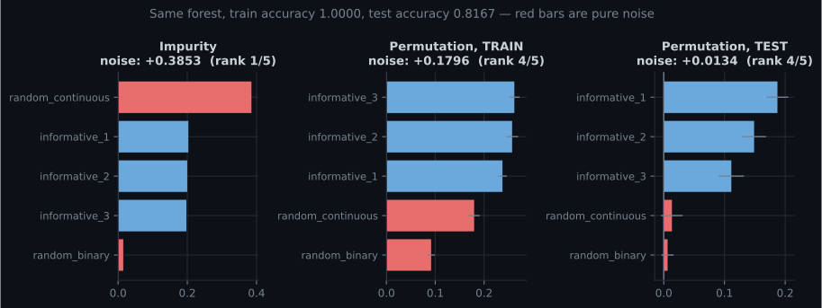
Thirty-eight percent of the model’s explanation, handed to a column that contains nothing. If you had used that ranking to decide which data to keep collecting, you would have invested in noise.

Why impurity importance does this

A decision tree splits by choosing the feature and threshold that most reduce impurity. feature_importances_feature_importances_ adds up, across every node in every tree, the impurity reduction each feature achieved, weighted by how many samples reached that node.

The problem is in the candidate set. For a binary feature there is exactly one possible split. For a continuous feature with $n$ distinct values there are $n - 1$. So the continuous column gets far more chances to find a threshold that happens to separate the training labels — and with enough candidates, one of them always will.

Two consequences follow directly from that formula:

It is measured on training data only. Every $\Delta i(t)$ is the impurity reduction the split achieved on the rows used to build the tree. A split that fits noise still reduces training impurity, and still gets credit.

It rewards cardinality. High-cardinality features win more splits. This is why the effect is strongest for continuous columns, unique IDs, timestamps and high-cardinality categoricals — and why random_binaryrandom_binary, which is equally uninformative, scored only 0.0148.

Note that the trap needs room to overfit. With clean labels and enough data the forest never has to reach for the noise column, and impurity importance looks fine. Here 10% of labels were flipped and train accuracy hit 1.0000 against a test accuracy of 0.8167 — that gap is the space in which the noise column got its 0.3853.

See it move

The mechanism is worth watching on twenty rows, because it needs no model at all. Below, labels are assigned at random and neither column carries a single bit of information about them. The continuous column wins anyway, because it gets $n - 1$ candidate thresholds to the binary column’s one — and the best of nineteen coin flips beats one coin flip. Over 20,000 samples of this exact setup the continuous column’s best Gini reduction averages 0.0836 against the binary column’s 0.0250, and it wins 89.1% of individual samples.

Let it run and the averages settle towards 0.0836 and 0.0250 — a 3.3× advantage on data where neither column knows anything. Scale that up to hundreds of nodes across three hundred trees, and you get 0.3853.

Permutation importance

The alternative asks a question that does not depend on how the model was built:

Shuffle one column. How much worse does the model get?

where $s$ is the score on intact data and $s_{\pi_k(f)}$ the score with feature $f$ randomly permuted, averaged over $K$ shuffles. Shuffling destroys the relationship between that column and the target while keeping its marginal distribution intact.

This is model-agnostic — it works on anything with a predictpredict method — and it measures what you usually want to know: how much the model relies on this column.

It must be computed on held-out data

This is the part that gets skipped, and the middle panel above shows why. On the training set the noise column scored +0.1796, because the forest genuinely does rely on it — to reproduce the memorised labels. Permuting it destroys that memorisation and the training score falls.

That is a true statement about the model and a useless one about the world.

# The default that hides the problem.
permutation_importance(model, X_train, y_train, n_repeats=30, random_state=0)
 
# What you almost always want instead.
permutation_importance(model, X_test, y_test, n_repeats=30, random_state=0)

# The default that hides the problem.
permutation_importance(model, X_train, y_train, n_repeats=30, random_state=0)
 
# What you almost always want instead.
permutation_importance(model, X_test, y_test, n_repeats=30, random_state=0)

Negative importance is meaningful

Permutation importance can come out below zero: the model got better with the column shuffled. That means the model was actively misled by it — it fitted a pattern that does not hold on new data.

A small negative value is noise; check it against importances_stdimportances_std. A consistently negative one is a feature worth deleting.

Correlated features split the credit

Second trap, and it bites even when you use permutation importance correctly on held-out data.

Take one genuine driver, incomeincome, plus a near-duplicate income_copyincome_copy (correlation ≈ 1), plus a weak independent feature.

figureSplit credit: neither column looks essential, and one of them ismatplotlib

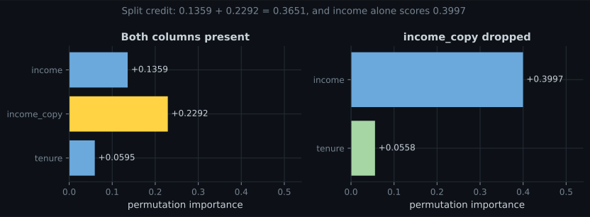
The mechanism is straightforward once you see it. Permuting incomeincome leaves income_copyincome_copy intact, so the model reads the signal from the copy and the score barely moves. Permuting income_copyincome_copy is symmetric. Each column individually looks dispensable, because each individually is — and together they are not.

Three practical consequences:

Never conclude “this feature does not matter” from a low permutation importance alone. Check its correlations first.

Cluster correlated features and permute the whole cluster together. Shuffling incomeincome and income_copyincome_copy simultaneously recovers the full 0.40.

Beware of dropping features by importance in a loop. Drop incomeincome because it scores 0.21, then re-measure, and income_copyincome_copy will now score 0.40 — you did no harm. Drop both in one pass because each scored low, and you have destroyed the model.

Which method for which question

That last row is deliberately blunt. feature_importances_feature_importances_ is fast, it is the default attribute, and it is the one people reach for. It is also the only method on this page that gave a badly wrong answer.

As a decision procedure rather than a table:

  flowchart TD
  Q["You want to say something
about a feature"] --> A{"About one row,
or about the model?"}
  A -->|"one row --
'why was I declined?'"| S["SHAP values"]
  A -->|"the model overall"| B{"Magnitude, or
direction and shape?"}
  B -->|"direction / shape"| P["PDP and ICE.
Check ICE spread before
trusting the average."]
  B -->|"magnitude / ranking"| C{"Are any features
correlated above ~0.8?"}
  C -->|"yes"| D["Cluster them first,
permute whole clusters.
Otherwise credit splits and
both look unimportant."]
  C -->|"no"| E{"Which question:
generalisation or fit?"}
  E -->|"generalisation --
what to keep collecting"| F["Permutation importance
on held-out data"]
  E -->|"fit -- overfitting
diagnostic"| G["Permutation importance
on training data.
Compare with the held-out run."]
  D --> F
  F --> H{"Does a feature you cannot
explain rank highly?"}
  H -->|"yes"| I["Suspect leakage or a shortcut
before celebrating."]
  H -->|"no"| J["Report the ranking with
its standard deviation
across repeats."]

Two branches carry the content of this page. The correlation check exists because permutation importance splits credit between duplicated columns, so two genuinely vital features can both score near zero. And the leakage check at the bottom is the one that saves projects: a high-ranking feature nobody can explain is a finding, not a result.

In code

import numpy as np
import pandas as pd
from sklearn.ensemble import RandomForestClassifier
from sklearn.inspection import permutation_importance
from sklearn.model_selection import train_test_split
 
rng = np.random.default_rng(0)
n = 1200
x1, x2 = rng.integers(0, 2, n), rng.integers(0, 2, n)
x3 = rng.integers(0, 3, n)
clean = ((x1 + x2 + (x3 > 1)) >= 2).astype(int)
y = np.where(rng.random(n) < 0.10, 1 - clean, clean)      # 10% label noise
 
X = pd.DataFrame({
    "informative_1": x1, "informative_2": x2, "informative_3": x3,
    "random_continuous": rng.normal(0, 1, n),             # pure noise, continuous
    "random_binary": rng.integers(0, 2, n),               # pure noise, binary
})
X_tr, X_te, y_tr, y_te = train_test_split(X, y, test_size=0.3, random_state=0,
                                          stratify=y)
model = RandomForestClassifier(n_estimators=300, random_state=0).fit(X_tr, y_tr)
print(f"train {model.score(X_tr, y_tr):.4f}  test {model.score(X_te, y_te):.4f}")
# train 1.0000  test 0.8167
 
for name, value in sorted(zip(X.columns, model.feature_importances_),
                          key=lambda t: -t[1]):
    print(f"  impurity  {name:20s} {value:.4f}")
# impurity  random_continuous    0.3853     <- pure noise, ranked FIRST
 
result = permutation_importance(model, X_te, y_te, n_repeats=30, random_state=0)
for i in np.argsort(-result.importances_mean):
    print(f"  perm/test {X.columns[i]:20s} "
          f"{result.importances_mean[i]:+.4f} +/- {result.importances_std[i]:.4f}")
# perm/test informative_1        +0.1872 +/- 0.0180
# perm/test random_continuous    +0.0134 +/- 0.0121     <- correctly near zero

import numpy as np
import pandas as pd
from sklearn.ensemble import RandomForestClassifier
from sklearn.inspection import permutation_importance
from sklearn.model_selection import train_test_split
 
rng = np.random.default_rng(0)
n = 1200
x1, x2 = rng.integers(0, 2, n), rng.integers(0, 2, n)
x3 = rng.integers(0, 3, n)
clean = ((x1 + x2 + (x3 > 1)) >= 2).astype(int)
y = np.where(rng.random(n) < 0.10, 1 - clean, clean)      # 10% label noise
 
X = pd.DataFrame({
    "informative_1": x1, "informative_2": x2, "informative_3": x3,
    "random_continuous": rng.normal(0, 1, n),             # pure noise, continuous
    "random_binary": rng.integers(0, 2, n),               # pure noise, binary
})
X_tr, X_te, y_tr, y_te = train_test_split(X, y, test_size=0.3, random_state=0,
                                          stratify=y)
model = RandomForestClassifier(n_estimators=300, random_state=0).fit(X_tr, y_tr)
print(f"train {model.score(X_tr, y_tr):.4f}  test {model.score(X_te, y_te):.4f}")
# train 1.0000  test 0.8167
 
for name, value in sorted(zip(X.columns, model.feature_importances_),
                          key=lambda t: -t[1]):
    print(f"  impurity  {name:20s} {value:.4f}")
# impurity  random_continuous    0.3853     <- pure noise, ranked FIRST
 
result = permutation_importance(model, X_te, y_te, n_repeats=30, random_state=0)
for i in np.argsort(-result.importances_mean):
    print(f"  perm/test {X.columns[i]:20s} "
          f"{result.importances_mean[i]:+.4f} +/- {result.importances_std[i]:.4f}")
# perm/test informative_1        +0.1872 +/- 0.0180
# perm/test random_continuous    +0.0134 +/- 0.0121     <- correctly near zero

Permuting a correlated group together:

import numpy as np
 
 
def grouped_permutation_importance(model, X, y, groups, n_repeats=30, seed=0):
    """Permute whole clusters of correlated columns at once."""
    rng = np.random.default_rng(seed)
    baseline = model.score(X, y)
    out = {}
    for label, cols in groups.items():
        drops = []
        for _ in range(n_repeats):
            X_shuffled = X.copy()
            order = rng.permutation(len(X))
            for c in cols:                        # SAME permutation for the group
                X_shuffled[c] = X[c].to_numpy()[order]
            drops.append(baseline - model.score(X_shuffled, y))
        out[label] = (float(np.mean(drops)), float(np.std(drops)))
    return out
 
 
groups = {"income (both columns)": ["income", "income_copy"], "tenure": ["tenure"]}

import numpy as np
 
 
def grouped_permutation_importance(model, X, y, groups, n_repeats=30, seed=0):
    """Permute whole clusters of correlated columns at once."""
    rng = np.random.default_rng(seed)
    baseline = model.score(X, y)
    out = {}
    for label, cols in groups.items():
        drops = []
        for _ in range(n_repeats):
            X_shuffled = X.copy()
            order = rng.permutation(len(X))
            for c in cols:                        # SAME permutation for the group
                X_shuffled[c] = X[c].to_numpy()[order]
            drops.append(baseline - model.score(X_shuffled, y))
        out[label] = (float(np.mean(drops)), float(np.std(drops)))
    return out
 
 
groups = {"income (both columns)": ["income", "income_copy"], "tenure": ["tenure"]}

Using one shared permutation for the whole group matters: independently shuffling each column would break their correlation, which changes the distribution the model sees and inflates the estimate.

Pitfalls

Using feature_importances_feature_importances_ for anything that matters. It gave rank 1 to pure Gaussian noise, with 38.53% of the total credit.

Computing permutation importance on training data. It rewards memorisation — the noise column scored +0.1796 there against +0.0134 on held-out data.

Concluding a feature is useless from a low permutation score. Check correlations. incomeincome scored 0.2089 with its duplicate present and 0.4009 without.

Dropping several low-importance features in one pass. Two correlated columns can each score low while the pair is essential.

Interpreting importance of a bad model. If test accuracy is near the baseline, the importances describe noise. Establish that the model works first.

Reading direction into importance. All these methods give magnitude only. “Income matters a lot” does not say whether more income raises or lowers the prediction — that needs PDP or SHAP.

Ignoring importances_stdimportances_std. A value of 0.02 ± 0.03 is indistinguishable from zero. The standard deviation is returned for a reason.

Recap

• feature_importances_feature_importances_ ranked a pure noise column first, at 0.3853 — because impurity importance is computed on training data and rewards high cardinality.
• The trap needs overfitting room: train 1.0000 against test 0.8167 is where the noise got its credit.
• Permutation importance is model-agnostic and asks the right question, but must be computed on held-out data — the same noise column scored +0.1796 on train.
• Negative permutation importance means the feature actively misleads the model.
• Correlated features split the credit: 0.2089 + 0.1489, and incomeincome alone scores 0.4009. Permute correlated clusters together.
• Every method here is global and unsigned. Direction needs PDP; per-row attribution needs SHAP.

🧪 Try It Yourself

Exercise 1 – Reproduce the trap

Exercise 2 – Permutation importance, train against test

Exercise 3 – Watch correlated features split the credit

Exercise 4 – Permute a correlated group together

Exercise 5 – Find a misleading feature

Next

Partial Dependence and ICE Plots — importance told you how much a feature matters. The next question is which direction, and the answer is where averaging becomes dangerous.