
Image Segmentation
Classification answers “what is in this image”. Segmentation answers “what is each pixel” — one label per position, at the input’s resolution. That changes the output shape, forces the network to recover spatial detail it deliberately threw away, and makes the obvious metric almost useless.
The data here is generated rather than downloaded: 1,200 training scenes of 64×64 containing a disc, a square and a triangle on noisy backgrounds, each with an exact per-pixel label map. Every mask is known to be correct, and the whole page runs on a CPU in a couple of minutes.
What you’ll learn
Section titled “What you’ll learn”- Why the output is with a softmax over the channel axis, not a single vector.
- The metric trap: predicting “background” everywhere scores 0.8691 pixel accuracy on this data.
- Three upsampling designs measured, where plain upsampling plus convolution won at 0.8965 mean IoU and transposed convolution with skips came last at 0.8001.
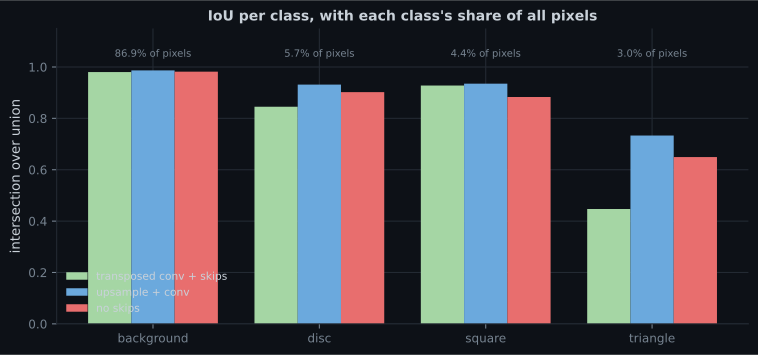
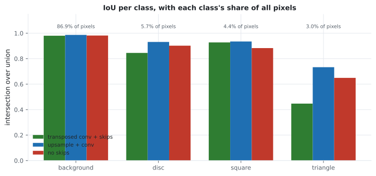
- Why the smallest class is always the worst: triangle IoU 0.4470 to 0.7331 while background sits above 0.98.
- What
Conv2DTransposedoes to a shape, and how it differs fromUpSampling2D. - Where segmentation errors actually live — the one-pixel boundary.
The output is an image
Section titled “The output is an image”A classifier ends with Dense(classes, activation="softmax") — one vector. A
segmentation model ends with Conv2D(classes, 1, activation="softmax") — one
vector per pixel, because a 1×1 convolution applied to an feature map
produces and the softmax runs along the last axis.
# classification
keras.layers.GlobalAveragePooling2D(),
keras.layers.Dense(4, activation="softmax")        # (4,)

# segmentation
keras.layers.Conv2D(4, 1, activation="softmax")    # (64, 64, 4)
The loss is unchanged. sparse_categorical_crossentropy against an integer mask of
shape averages the per-pixel loss over every position — 4,096 predictions
per image instead of one.
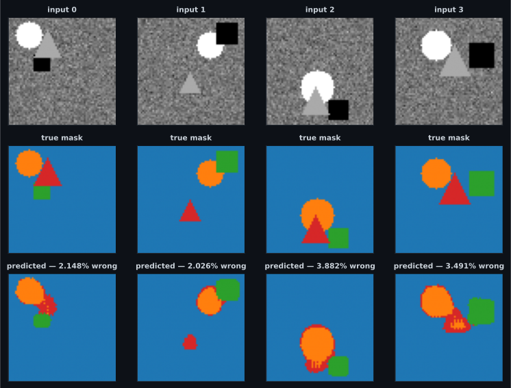
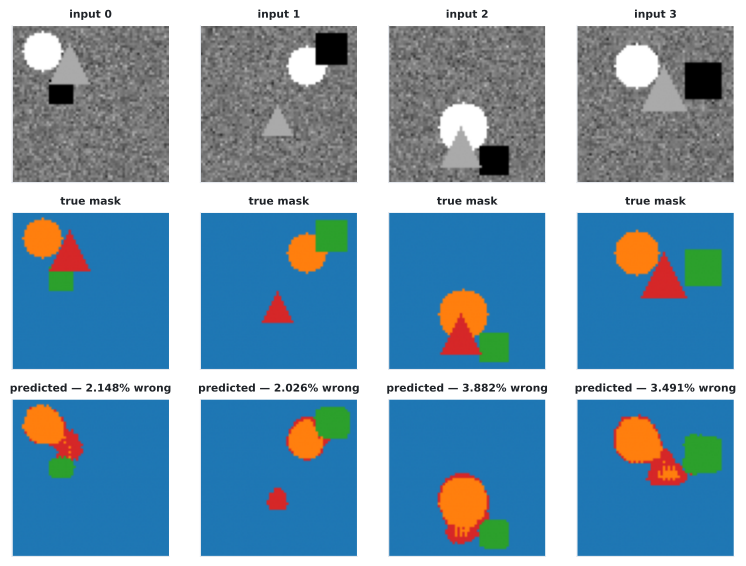
The metric trap
Section titled “The metric trap”| Class | Share of all pixels |
|---|---|
| background | 0.8691 |
| disc | 0.0568 |
| square | 0.0438 |
| triangle | 0.0303 |
A model that outputs “background” for every pixel scores 0.8691 pixel accuracy and is completely useless. The trained model’s 0.9737 is only 0.10 above that baseline — the same imbalance problem measured on the Reuters page, except that in segmentation it is structural: backgrounds are always most of the image.
The standard fix is intersection over union, per class:
The all-background model scores IoU 0.8691 on background and exactly 0.0 on the other three, for a mean IoU of 0.2173. That is the number that tells you the model does nothing.
  flowchart LR
  A["input 64x64x1"] --> B["Conv 16
64x64"]
  B --> C["pool
32x32"]
  C --> D["Conv 32
32x32"]
  D --> E["pool
16x16"]
  E --> F["Conv 64
16x16
widest view"]
  F --> G["upsample
32x32"]
  G --> H["upsample
64x64"]
  H --> I["Conv2D(4, 1)
softmax per pixel"]
  B -. "skip: 64x64 detail" .-> H
  D -. "skip: 32x32 detail" .-> G
The shape is an hourglass: downsample to see context, upsample to recover position. The skip connections exist because the downsampling path destroys the precise location of every boundary, and the upsampling path cannot invent it back.
Getting the resolution back
Section titled “Getting the resolution back”Three ways, measured on identical data with the same seed:
| Design | Parameters | Pixel accuracy | Mean IoU | Seconds |
|---|---|---|---|---|
| transposed conv + skips | 51,124 | 0.9737 | 0.8001 | 72.8 |
| upsample + conv + skips | 51,124 | 0.9863 | 0.8965 | 219.3 |
| transposed conv, no skips | 46,452 | 0.9805 | 0.8540 | 77.8 |
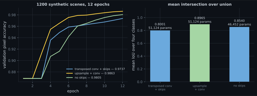
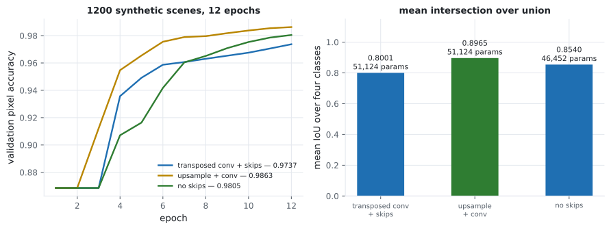
Two results here are worth stating carefully, because both contradict the usual advice:
- Plain upsampling plus a convolution beat transposed convolution at an
identical parameter count — 0.8965 against 0.8001 mean IoU.
UpSampling2Drepeats each value into a 2×2 block and the following convolution smooths it;Conv2DTransposelearns the upsampling, and here that flexibility cost more than it bought. It was also 3× slower in wall-clock, which is the opposite of what its simplicity suggests. - Dropping the skip connections beat one of the designs that used them — 0.8540 against 0.8001. That is not evidence against skip connections; it is evidence that this particular transposed-convolution decoder was the weak link, and the comparison only separates them because IoU is sensitive enough to notice.
The honest summary: on this problem the decoder choice mattered more than the skip connections, and the cheapest decoder won. Exercise 5 isolates it — the same upsample-plus-convolution decoder with and without skips scored 0.8965 and 0.8974 mean IoU, a difference of 0.0009 that is indistinguishable from run-to-run noise. On real segmentation tasks with thin structure — vessels, wires, text strokes — the skip connections matter much more than they do on four solid geometric shapes with clean boundaries, because there the boundary is the object.
What each upsampling layer actually does
Section titled “What each upsampling layer actually does”| Layer | (16, 16, 8) becomes | Parameters |
|---|---|---|
UpSampling2D(2) | (32, 32, 8) | 0 |
Conv2DTranspose(4, 3, strides=2) | (32, 32, 4) | 292 |
UpSampling2D(2) + Conv2D(4, 3) | (32, 32, 4) | 292 |
UpSampling2D is a fixed rule — nearest-neighbour repetition, no weights at all.
Conv2DTranspose inserts zeros between the input values and convolves, which is
mathematically the gradient of a strided convolution and is why it is sometimes
called a deconvolution (it is not one). The third row is the combination that won
above: fixed upsampling, then a learned smoothing.
Where the errors are
Section titled “Where the errors are”| Design | background | disc | square | triangle |
|---|---|---|---|---|
| transposed conv + skips | 0.9802 | 0.8453 | 0.9279 | 0.4470 |
| upsample + conv | 0.9866 | 0.9314 | 0.9351 | 0.7331 |
| no skips | 0.9817 | 0.9020 | 0.8830 | 0.6493 |
The triangle loses on two counts, and they compound:
- It is the smallest class at 3.0% of pixels, so it contributes almost nothing to the loss. A model can ignore it and still report 97% pixel accuracy.
- It has the most boundary per unit area. IoU on a small object is dominated by its outline: a shape 15 pixels across has roughly 56 boundary pixels out of 225 total, and a one-pixel error all the way round drops its IoU to 0.60.
That second point is the general rule of segmentation: the metric is decided at the boundaries, and small objects are almost all boundary. Weighting the loss by inverse class frequency, or using a Dice/IoU-based loss directly, is the standard response.
Pitfalls
Section titled “Pitfalls”- Reporting pixel accuracy. All-background scored 0.8691 here; the trained model scored 0.9737. The interesting information is in the 0.10 between them.
- Averaging IoU over pixels instead of classes. That reintroduces exactly the imbalance IoU was chosen to remove.
- Assuming
Conv2DTransposebeatsUpSampling2D+Conv2D. Measured 0.8001 against 0.8965 at identical parameter counts, and 3× slower. - Calling
Conv2DTransposea deconvolution. It is the gradient of a strided convolution, not an inverse; it cannot recover information the pooling discarded. - Omitting skip connections on fine structure. They cost nothing at inference and carry the boundary detail — on shapes this simple the decoder mattered more, which will not generalise to real images.
- Ignoring the smallest class. Triangle IoU ran 0.4470–0.7331 while background sat above 0.98, and the loss barely notices.
- Mismatching the mask encoding and the loss. An integer mask pairs with
sparse_categorical_crossentropy; an one-hot mask pairs withcategorical_crossentropy.
- Segmentation replaces the dense head with
Conv2D(classes, 1, activation="softmax")— one softmax vector per pixel, 4,096 predictions per 64×64 image. - Background was 86.91% of pixels, so a do-nothing model scores 0.8691 pixel accuracy and 0.2173 mean IoU. Report IoU.
- Three decoders at 12 epochs: upsample+conv 0.8965 mean IoU, no-skips 0.8540, transposed conv + skips 0.8001.
UpSampling2Dhas zero parameters;Conv2DTransposelearns the upsampling and was both worse and slower here.- Per-class IoU followed pixel share exactly, with triangle (3.0% of pixels) at 0.4470–0.7331 against background above 0.98.
- IoU on small objects is dominated by boundary pixels, which is why class weighting or a Dice-style loss is standard.
One label per pixel is one way to answer “where”. Boxes are the other, and they bring a different set of problems: Object Detection (Bounding Boxes and YOLO).
-
Your segmentation model reports 0.97 pixel accuracy. What is the first thing to check?
The all-background prediction also scores 0.0 IoU on every foreground class, for a mean IoU of 0.2173 — which is the number that reveals it.
pch.quizShowAnswer
B — What a do-nothing model scores — background was 86.91% of pixels here, so 0.8691 comes free and 0.97 is only 0.10 above it — The all-background prediction also scores 0.0 IoU on every foreground class, for a mean IoU of 0.2173 — which is the number that reveals it.
-
Plain UpSampling2D followed by Conv2D reached 0.8965 mean IoU while Conv2DTranspose with the same parameter count reached 0.8001. What does that suggest?
The same phase measured strided convolution losing to fixed pooling for downsampling. Extra flexibility costs parameters and optimisation difficulty.
pch.quizShowAnswer
B — A learned upsampler is not automatically better than a fixed rule plus a learned smoothing — and here the fixed-rule version was also three times faster in wall-clock — The same phase measured strided convolution losing to fixed pooling for downsampling. Extra flexibility costs parameters and optimisation difficulty.
-
Why is the triangle's IoU (0.4470 to 0.7331) so much worse than the background's (above 0.98)?
Both effects push the same way, which is why inverse-frequency weighting or a Dice-style loss is the standard response.
pch.quizShowAnswer
B — It is the smallest class at 3.0% of pixels, so it barely affects the loss, and small objects are mostly boundary — a one-pixel error round the outline of a 15-pixel shape drops its IoU to about 0.60 — Both effects push the same way, which is why inverse-frequency weighting or a Dice-style loss is the standard response.
-
What is the output layer of a four-class segmentation model on 64x64 inputs?
A 1x1 convolution is a per-pixel dense layer. The loss then averages cross-entropy over all 4,096 positions.
pch.quizShowAnswer
B — Conv2D(4, 1, activation='softmax'), producing (64, 64, 4) — one softmax vector per pixel, with the softmax along the channel axis — A 1x1 convolution is a per-pixel dense layer. The loss then averages cross-entropy over all 4,096 positions.
-
Conv2DTranspose is often called a deconvolution. Why is that name wrong?
Nothing in the upsampling path can invent back a boundary position that the downsampling path destroyed. The skip connection carries it forward instead.
pch.quizShowAnswer
B — Because it is the gradient of a strided convolution, not its inverse — it cannot recover information that pooling discarded, which is exactly why skip connections exist — Nothing in the upsampling path can invent back a boundary position that the downsampling path destroyed. The skip connection carries it forward instead.
🧪 Try It Yourself
Section titled “🧪 Try It Yourself”pch.coffeeTagline
pch.coffeeCtapch.feedbackHeading
pch.feedbackSubheading