Matrices

A matrix is a rectangular grid of numbers. That sounds humble, but it is the single most important object in machine learning, and the reason is that it has two faces. A matrix can be data — a spreadsheet, an image, a batch of feature vectors — and it can be an action: a rotation, a projection, a neural network layer.

The book says this outright at the top of §2.2: matrices “can be used to compactly represent systems of linear equations, but they also represent linear functions”. Learning to switch between those two readings, and to know which one a given page means, is the skill this section buys you.

What you’ll learn

• What a matrix is, precisely, and why $\mathbb{R}^{m\times n}$ can be treated as $\mathbb{R}^{mn}$.
• Why multiplication is not element-wise, and what it is instead.
• The one idea that makes matrix multiplication obvious: the columns are the images of the basis vectors.
• Why $\mathbf{A}\mathbf{B} \neq \mathbf{B}\mathbf{A}$, and why even their shapes can differ.
• Identity, inverse, transpose, symmetry — and the four look-alike identities that are false.

Intuition: a grayscale image, and a machine that bends the plane

Open any grayscale photo, zoom in far enough, and you find a grid of brightness values from 0 to 255. A 1080×1920 photo is a matrix with 1080 rows and 1920 columns. Every filter you have used — blur, sharpen, edge-detect — is arithmetic on that grid. Matrix as data.

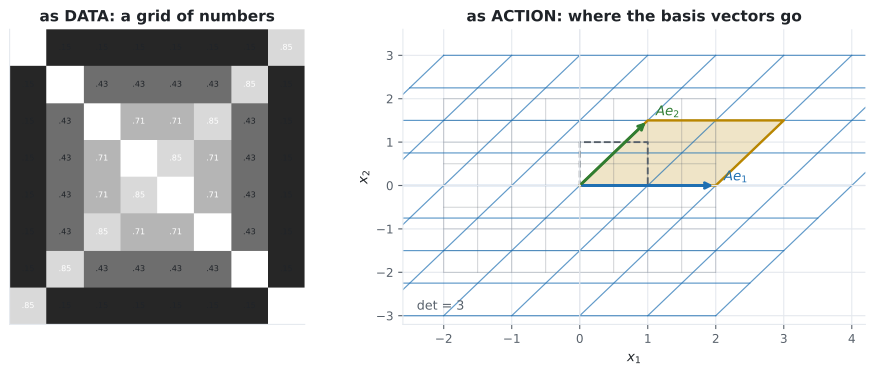
Now take the tiny matrix $\begin{bmatrix}2 & 1\\ 0 & 1.5\end{bmatrix}$ and multiply every point of a sheet of graph paper by it. The grid stretches and shears into a new grid — still straight lines, still evenly spaced, but tilted. Matrix as action.

diagram Diagram mermaid

  flowchart TD
  M["a matrix"]
  M --> D["DATA
rows are observations,
columns are features"]
  M --> A["ACTION
a linear map that sends
the basis vectors somewhere"]
  D --> D1["an image, a design matrix,
a batch of embeddings"]
  A --> A1["rotation, projection,
a neural network layer"]
  A --> A2["its COLUMNS are exactly
where the basis vectors land"]
  A2 --> KEY["so multiplication is
composition of actions,
not entry-by-entry arithmetic"]

The right-hand branch is the whole page. Once you believe the columns are the images of the basis vectors, the multiplication rule stops being a formula to memorise and becomes the only rule it could possibly be.

The math

Definition

A real-valued $(m, n)$ matrix $\mathbf{A}$ has $m$ rows and $n$ columns:

$$\mathbf{A} = \begin{bmatrix} a_{11} & a_{12} & \cdots & a_{1n}\\ a_{21} & a_{22} & \cdots & a_{2n}\\ \vdots & \vdots & \ddots & \vdots\\ a_{m1} & a_{m2} & \cdots & a_{mn} \end{bmatrix}, \qquad a_{ij} \in \mathbb{R}.$$

The entry $a_{ij}$ sits in row $i$, column $j$ — row index always first. A $(1, n)$ matrix is a row vector; an $(m, 1)$ matrix is a column vector. The set of all real $(m,n)$ matrices is $\mathbb{R}^{m\times n}$.

The book adds a remark that pays off later: by stacking its columns into one long vector, any $\mathbf{A} \in \mathbb{R}^{m\times n}$ can be represented as a vector in $\mathbb{R}^{mn}$. So $\mathbb{R}^{m\times n}$ and $\mathbb{R}^{mn}$ are “the same” as vector spaces — a claim §2.7 makes precise via Theorem 2.17 (equal dimension implies isomorphic). It is also exactly what A.reshape(-1) does, and why a weight matrix can be handed to an optimiser as a flat parameter vector.

Addition and scaling: element by element

Two matrices of the same shape add entry-by-entry, and $\lambda\mathbf{A}$ multiplies every entry by $\lambda$. No surprises, and both are exactly what NumPy’s + and * do.

That is worth flagging, because it sets up the trap: addition is element-wise and multiplication is not. The operator that looks most similar behaves least similarly.

Multiplication: the one that trips everyone

To multiply $\mathbf{A} \in \mathbb{R}^{m\times n}$ by $\mathbf{B} \in \mathbb{R}^{n\times k}$, each entry of $\mathbf{C} = \mathbf{A}\mathbf{B}$ is a dot product of a row of $\mathbf{A}$ with a column of $\mathbf{B}$:

$$c_{ij} = \sum_{l=1}^{n} a_{il}\, b_{lj}, \qquad i = 1,\dots,m,\;\; j = 1,\dots,k.$$

The neighbouring dimensions must match — columns of $\mathbf{A}$ equals rows of $\mathbf{B}$ — and the result takes the outer dimensions:

$$\underbrace{\mathbf{A}}_{m\times n}\underbrace{\mathbf{B}}_{n\times k} = \underbrace{\mathbf{C}}_{m\times k}$$

This is not the element-wise product

The element-wise product $c_{ij} = a_{ij}b_{ij}$ is a different operation with its own name — the Hadamard product — and the book calls it out explicitly because “this kind of element-wise multiplication often appears in programming languages when we multiply multi-dimensional arrays”.

In NumPy, A @ B is the matrix product and A * B is the Hadamard product. Both run. Both return an array of a plausible shape. Only one is the mathematics on this page. See NumPy for Mathematics for why this is the most expensive typo in numerical Python.

Why that rule, and not some other one?

Because multiplication is composition. Applying $\mathbf{B}$ and then $\mathbf{A}$ should be the same as applying the single matrix $\mathbf{A}\mathbf{B}$, and that requirement forces the formula.

Here is the argument in one line. The $j$-th column of any matrix $\mathbf{M}$ is $\mathbf{M}\mathbf{e}_j$ — the image of the $j$-th basis vector. So the $j$-th column of $\mathbf{A}\mathbf{B}$ must be

$$(\mathbf{A}\mathbf{B})\mathbf{e}_j = \mathbf{A}(\mathbf{B}\mathbf{e}_j) = \mathbf{A}\,(\text{$j$-th column of }\mathbf{B}),$$

which is a weighted sum of $\mathbf{A}$‘s columns with weights from $\mathbf{B}$‘s $j$-th column — precisely $\sum_l a_{il}b_{lj}$. The rule is not a convention; it is the only rule under which “multiply the matrices” means “do one thing then the other”.

This also explains the dimension requirement without any memorisation: $\mathbf{B}$ outputs vectors in $\mathbb{R}^n$, so $\mathbf{A}$ must accept vectors in $\mathbb{R}^n$, so $\mathbf{A}$ must have $n$ columns.

Order matters, and so does shape

$$\mathbf{A}\mathbf{B} \neq \mathbf{B}\mathbf{A} \quad\text{in general}$$

Obvious once you think of composition: rotating then stretching is not stretching then rotating. But the book makes a sharper point with its Figure 2.5 — even when both products are defined, their shapes can differ. With $\mathbf{A}$ being $2\times3$ and $\mathbf{B}$ being $3\times2$, $\mathbf{A}\mathbf{B}$ is $2\times2$ and $\mathbf{B}\mathbf{A}$ is $3\times3$. They are not merely unequal; they do not live in the same space.

What does hold:

$$(\mathbf{A}\mathbf{B})\mathbf{C} = \mathbf{A}(\mathbf{B}\mathbf{C}), \qquad (\mathbf{A}+\mathbf{B})\mathbf{C} = \mathbf{A}\mathbf{C} + \mathbf{B}\mathbf{C}, \qquad \mathbf{A}(\mathbf{C}+\mathbf{D}) = \mathbf{A}\mathbf{C} + \mathbf{A}\mathbf{D}$$

Associativity is why (A @ B) @ C and A @ (B @ C) agree mathematically — though they can differ wildly in cost, which is the whole subject of optimising a chain of matrix products.

Identity, inverse, transpose

The identity $\mathbf{I}_n$ has ones on the diagonal and zeros elsewhere, and $\mathbf{I}_m\mathbf{A} = \mathbf{A}\mathbf{I}_n = \mathbf{A}$. Note the two different sizes: for a non-square $\mathbf{A}$ the left and right identities are different matrices.

An inverse $\mathbf{A}^{-1}$ satisfies

$$\mathbf{A}\mathbf{A}^{-1} = \mathbf{I} = \mathbf{A}^{-1}\mathbf{A},$$

and only square matrices can have one. When it exists $\mathbf{A}$ is called regular, invertible or nonsingular; when it does not, singular or noninvertible. The book notes the inverse is unique when it exists — so “the” inverse is well defined.

For $2\times2$ there is a closed form worth knowing:

$$\mathbf{A} = \begin{bmatrix} a_{11} & a_{12}\\ a_{21} & a_{22}\end{bmatrix} \quad\Longrightarrow\quad \mathbf{A}^{-1} = \frac{1}{a_{11}a_{22} - a_{12}a_{21}}\begin{bmatrix} a_{22} & -a_{12}\\ -a_{21} & a_{11}\end{bmatrix}$$

valid if and only if $a_{11}a_{22} - a_{12}a_{21} \neq 0$. That quantity is the determinant (§4.1), and this is the first place it appears: as the thing that must not be zero.

The transpose $\mathbf{A}^\top$ has $b_{ij} = a_{ji}$ — the columns of $\mathbf{A}$ written as the rows of $\mathbf{A}^\top$. A matrix is symmetric when $\mathbf{A} = \mathbf{A}^\top$, which only a square matrix can be.

The four identities that are true, and the two that are not

$$\begin{aligned} (\mathbf{A}\mathbf{B})^{-1} &= \mathbf{B}^{-1}\mathbf{A}^{-1} &&\text{\textbf{true} — note the order flips}\\ (\mathbf{A}\mathbf{B})^\top &= \mathbf{B}^\top\mathbf{A}^\top &&\text{\textbf{true} — order flips here too}\\ (\mathbf{A}^\top)^\top &= \mathbf{A} &&\text{\textbf{true}}\\ (\mathbf{A}+\mathbf{B})^\top &= \mathbf{A}^\top + \mathbf{B}^\top &&\text{\textbf{true}}\\[6pt] (\mathbf{A}+\mathbf{B})^{-1} &\neq \mathbf{A}^{-1} + \mathbf{B}^{-1} &&\text{\textbf{FALSE}} \end{aligned}$$

The book gives the one-number sanity check for the false one: the scalar case is $\tfrac{1}{2+4} = \tfrac16 \neq \tfrac12 + \tfrac14$. If it fails for numbers it fails for matrices.

And a second false-looking-true claim: the sum of two symmetric matrices is always symmetric, but their product generally is not. The book’s counterexample is worth keeping:

$$\begin{bmatrix}1 & 0\\ 0 & 0\end{bmatrix}\begin{bmatrix}1 & 1\\ 1 & 1\end{bmatrix} = \begin{bmatrix}1 & 1\\ 0 & 0\end{bmatrix}$$

Both factors are symmetric; the product is not. This matters more than it looks: covariance matrices are symmetric and products of them appear constantly, so assuming symmetry survives multiplication is a real bug waiting to happen. (It does survive in the special form $\mathbf{A}^\top\mathbf{A}$, which is always symmetric — the fact §3.8 and Chapter 9 rely on.)

Worked example by hand

The book’s Example 2.3, computed entry by entry. With

$$\mathbf{A} = \begin{bmatrix}1 & 2 & 3\\ 3 & 2 & 1\end{bmatrix} \in \mathbb{R}^{2\times3}, \qquad \mathbf{B} = \begin{bmatrix}0 & 2\\ 1 & -1\\ 0 & 1\end{bmatrix} \in \mathbb{R}^{3\times2}$$

$\mathbf{A}\mathbf{B}$ is $2\times2$. Each entry is one dot product:

entry	row of $\mathbf{A}$	column of $\mathbf{B}$	arithmetic	value
$c_{11}$	$(1, 2, 3)$	$(0, 1, 0)$	$1\cdot0 + 2\cdot1 + 3\cdot0$	$2$
$c_{12}$	$(1, 2, 3)$	$(2, -1, 1)$	$1\cdot2 + 2\cdot(-1) + 3\cdot1$	$3$
$c_{21}$	$(3, 2, 1)$	$(0, 1, 0)$	$3\cdot0 + 2\cdot1 + 1\cdot0$	$2$
$c_{22}$	$(3, 2, 1)$	$(2, -1, 1)$	$3\cdot2 + 2\cdot(-1) + 1\cdot1$	$5$

$$\mathbf{A}\mathbf{B} = \begin{bmatrix}2 & 3\\ 2 & 5\end{bmatrix}$$

Now the other order. $\mathbf{B}\mathbf{A}$ is $3\times3$ — a different shape entirely:

$$\mathbf{B}\mathbf{A} = \begin{bmatrix}6 & 4 & 2\\ -2 & 0 & 2\\ 3 & 2 & 1\end{bmatrix}$$

Spot-checking two entries: the $(1,1)$ entry is $(0,2)\cdot(1,3) = 0 + 6 = 6$ ✓, and the $(2,3)$ entry is $(1,-1)\cdot(3,1) = 3 - 1 = 2$ ✓.

And a $2\times2$ inverse by the formula. For $\mathbf{A} = \begin{bmatrix}4 & 1\\ 2 & 2\end{bmatrix}$ the determinant is $4\cdot2 - 1\cdot2 = 6$, so

$$\mathbf{A}^{-1} = \frac{1}{6}\begin{bmatrix}2 & -1\\ -2 & 4\end{bmatrix} = \begin{bmatrix}0.\overline{3} & -0.1\overline{6}\\ -0.\overline{3} & 0.\overline{6}\end{bmatrix}$$

Check: $\begin{bmatrix}4&1\\2&2\end{bmatrix}\cdot\tfrac16\begin{bmatrix}2&-1\\-2&4\end{bmatrix} = \tfrac16\begin{bmatrix}8-2 & -4+4\\ 4-4 & -2+8\end{bmatrix} = \tfrac16\begin{bmatrix}6&0\\0&6\end{bmatrix} = \mathbf{I}$ ✓

See it move

The lab below builds the action of a $2\times2$ matrix one column at a time. Frames 2 and 3 place the images of $\mathbf{e}_1$ and $\mathbf{e}_2$ — which are the columns — and everything after them follows by linearity.

matrixA matrix is just where the basis vectors golinear map on R^2

2101.50

columns of A = images of e1, e2

det A 3area factor 3orientation preserved

1e1, e2 = (1, 0), (0, 1)          # the basis we start from2A @ e1  ==  A[:, 0]              # first column IS the image of e13A @ e2  ==  A[:, 1]              # second column IS the image of e24# linearity: A(x1 e1 + x2 e2) = x1 (A e1) + x2 (A e2)5det(A) = a*d - b*c               # signed area of the image of the unit square6A @ v = lam * v                  # an eigenvector keeps its direction

det A3A e1(2, 0)A e2(1, 1.50)

basisThe plane before anything happens, with the standard basis e1 = (1, 0) and e2 = (0, 1) and the unit square they span.

Play‹›1/8⟲

The dashed square is the unit square before the map; the amber parallelogram is its image, and its area is the determinant.

Watch the probe frame in particular. It computes $1\cdot\mathbf{A}\mathbf{e}_1 + 1\cdot\mathbf{A}\mathbf{e}_2$ and lands on exactly the same point as $\mathbf{A}(1,1)^\top$ — because it is the same computation. That is linearity, and it is why knowing two columns tells you the whole map.

And a singular one, where the two columns are multiples of each other:

matrixA singular matrix collapses the plane onto a linelinear map on R^2

2142

columns of A = images of e1, e2

det A 0area factor 0orientation collapsed

1e1, e2 = (1, 0), (0, 1)          # the basis we start from2A @ e1  ==  A[:, 0]              # first column IS the image of e13A @ e2  ==  A[:, 1]              # second column IS the image of e24# linearity: A(x1 e1 + x2 e2) = x1 (A e1) + x2 (A e2)5det(A) = a*d - b*c               # signed area of the image of the unit square6A @ v = lam * v                  # an eigenvector keeps its direction

det A0A e1(2, 4)A e2(1, 2)

basisThe plane before anything happens, with the standard basis e1 = (1, 0) and e2 = (0, 1) and the unit square they span.

Play‹›1/7⟲

Both columns point the same way, so the image of the unit square has zero area. Nothing that lands on that line remembers where it came from.

The parallelogram has collapsed to a segment: determinant zero, no inverse. Information has been destroyed, and no matrix can undo that — which is the geometric content of “singular”.

From scratch

matrices.py

import numpy as np
 
# ---- the book's Example 2.3 ---------------------------------------------
A = np.array([[1.0, 2.0, 3.0],
              [3.0, 2.0, 1.0]])          # 2x3
B = np.array([[0.0,  2.0],
              [1.0, -1.0],
              [0.0,  1.0]])              # 3x2
 
print("A @ B =\n", A @ B, "  shape", (A @ B).shape)
print("B @ A =\n", B @ A, "  shape", (B @ A).shape)
print("same shape?", (A @ B).shape == (B @ A).shape)
 
# ---- multiplication IS composition -------------------------------------
# The j-th column of A@B equals A applied to the j-th column of B.
for j in range(B.shape[1]):
    print(f"col {j}: (A@B)[:,{j}] =", (A @ B)[:, j], " A @ B[:,{}] =".format(j), A @ B[:, j])
 
# ---- the columns are the images of the basis vectors --------------------
M = np.array([[2.0, 1.0], [0.0, 1.5]])
e1, e2 = np.array([1.0, 0.0]), np.array([0.0, 1.0])
print("\nM @ e1 =", M @ e1, " == first column ", M[:, 0])
print("M @ e2 =", M @ e2, " == second column", M[:, 1])
print("linearity: M @ (e1+e2) == M@e1 + M@e2 :", np.allclose(M @ (e1 + e2), M @ e1 + M @ e2))
 
# ---- @ versus * ---------------------------------------------------------
P = np.array([[1.0, 2.0], [3.0, 4.0]])
Q = np.array([[5.0, 6.0], [7.0, 8.0]])
print("\nP @ Q (matrix product):\n", P @ Q)
print("P * Q (Hadamard)      :\n", P * Q)
 
# ---- inverse, by formula and by library --------------------------------
A2 = np.array([[4.0, 1.0], [2.0, 2.0]])
det = A2[0, 0] * A2[1, 1] - A2[0, 1] * A2[1, 0]
by_hand = np.array([[A2[1, 1], -A2[0, 1]], [-A2[1, 0], A2[0, 0]]]) / det
print("\ndet =", det)
print("inverse by formula:\n", np.round(by_hand, 6))
print("matches np.linalg.inv:", np.allclose(by_hand, np.linalg.inv(A2)))
print("A @ A^-1 == I:", np.allclose(A2 @ by_hand, np.eye(2)))
 
# ---- the book's Example 2.4: a 3x3 inverse pair ------------------------
A3 = np.array([[1.0, 2.0, 1.0], [4.0, 4.0, 5.0], [6.0, 7.0, 7.0]])
B3 = np.array([[-7.0, -7.0, 6.0], [2.0, 1.0, -1.0], [4.0, 5.0, -4.0]])
print("\nExample 2.4: A@B == I:", np.allclose(A3 @ B3, np.eye(3)),
      " B@A == I:", np.allclose(B3 @ A3, np.eye(3)))
 
# ---- the identities: which hold and which do not ----------------------
R = np.array([[2.0, 1.0], [1.0, 3.0]])
S = np.array([[1.0, 0.0], [2.0, 1.0]])
print("\n(RS)^T == S^T R^T        :", np.allclose((R @ S).T, S.T @ R.T))
print("(RS)^-1 == S^-1 R^-1     :", np.allclose(np.linalg.inv(R @ S),
                                                np.linalg.inv(S) @ np.linalg.inv(R)))
print("(R+S)^-1 == R^-1 + S^-1  :", np.allclose(np.linalg.inv(R + S),
                                                np.linalg.inv(R) + np.linalg.inv(S)))
print("scalar check 1/(2+4) vs 1/2+1/4:", 1 / (2 + 4), "vs", 1 / 2 + 1 / 4)
 
# ---- symmetry does not survive multiplication -------------------------
X = np.array([[1.0, 0.0], [0.0, 0.0]])
Y = np.array([[1.0, 1.0], [1.0, 1.0]])
XY = X @ Y
print("\nX symmetric:", np.allclose(X, X.T), " Y symmetric:", np.allclose(Y, Y.T))
print("X@Y =\n", XY, "\nX@Y symmetric:", np.allclose(XY, XY.T))
print("but A^T A always is:", np.allclose(A.T @ A, (A.T @ A).T))
 
# ---- stacking columns: R^{m x n} is R^{mn} ----------------------------
flat = A.reshape(-1, order="F")           # column-major, as the book stacks
print("\nA shape", A.shape, "-> flattened", flat.shape, ":", flat)

text

A @ B =
 [[2. 3.]
 [2. 5.]]   shape (2, 2)
B @ A =
 [[ 6.  4.  2.]
 [-2.  0.  2.]
 [ 3.  2.  1.]]   shape (3, 3)
same shape? False
col 0: (A@B)[:,0] = [2. 2.]  A @ B[:,0] = [2. 2.]
col 1: (A@B)[:,1] = [3. 5.]  A @ B[:,1] = [3. 5.]
 
M @ e1 = [2. 0.]  == first column  [2. 0.]
M @ e2 = [1.  1.5]  == second column [1.  1.5]
linearity: M @ (e1+e2) == M@e1 + M@e2 : True
 
P @ Q (matrix product):
 [[19. 22.]
 [43. 50.]]
P * Q (Hadamard)      :
 [[ 5. 12.]
 [21. 32.]]
 
det = 6.0
inverse by formula:
 [[ 0.333333 -0.166667]
 [-0.333333  0.666667]]
matches np.linalg.inv: True
A @ A^-1 == I: True
 
Example 2.4: A@B == I: True  B@A == I: True
 
(RS)^T == S^T R^T        : True
(RS)^-1 == S^-1 R^-1     : True
(R+S)^-1 == R^-1 + S^-1  : False
scalar check 1/(2+4) vs 1/2+1/4: 0.16666666666666666 vs 0.75
 
X symmetric: True  Y symmetric: True
X@Y =
 [[1. 1.]
 [0. 0.]]
X@Y symmetric: False
but A^T A always is: True
 
A shape (2, 3) -> flattened (6,) : [1. 3. 2. 2. 3. 1.]

Three lines to notice. The same shape? False line is the book’s Figure 2.5 point: both products exist and they are not even comparable. The col 0 lines confirm multiplication is composition, column by column. And the scalar check, 0.1666… vs 0.75, is a one-second refutation of the inverse-of-a-sum identity — if it fails for numbers, do not bother testing matrices.

On real data

figure The same object, read two ways matplotlib

Left, the matrix is what is being looked at. Right, the matrix is what is doing the looking. Nothing about the numbers changes.

figure The same arithmetic, four orders of magnitude apart matplotlib

Both follow the n-cubed reference slope, so the algorithm is the same. The gap is constant factors — BLAS, cache blocking and vectorisation.

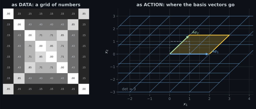
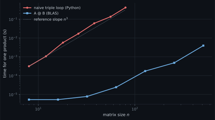
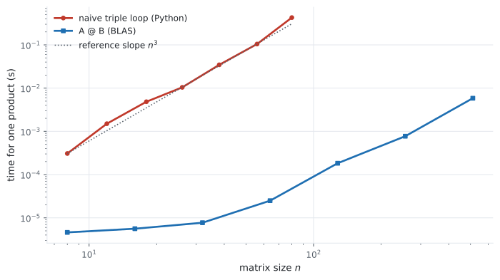
Reading the plot

The second figure makes a point that is easy to state and easy to forget. Both curves are parallel to the $n^3$ reference line, so the naive loop and @ are doing the same number of arithmetic operations. The four-orders-of-magnitude gap is entirely constant factors: a tuned BLAS keeps the working set in cache, issues vector instructions, and never touches the Python interpreter.

The lesson is not “NumPy is faster”. It is that asymptotic complexity and wall-clock time are different questions, and for matrix work the constants are large enough to decide whether an experiment finishes today. It is also why §2.3 remarks that Gaussian elimination is “impractical” at scale despite being perfectly correct: cubic is cubic, whoever writes the loop.

From the book

Mathematics for Machine Learning §2.2 opens by noting that matrices both represent systems of linear equations and represent linear functions (§2.7). Definition 2.1 gives the $(m,n)$ matrix (Equation 2.11) and the row/column-vector convention; the remark after it, with Figure 2.4, notes that stacking the $n$ columns represents $\mathbf{A} \in \mathbb{R}^{m\times n}$ as a vector in $\mathbb{R}^{mn}$. Addition is Equation 2.12 and multiplication Equation 2.13, with the remark that “neighbouring” dimensions must match (Equation 2.14) and that the element-wise product is a different operation called the Hadamard product. Example 2.3 computes both $\mathbf{A}\mathbf{B} = \begin{bmatrix}2&3\\2&5\end{bmatrix}$ (Equation 2.15) and $\mathbf{B}\mathbf{A}$ as a $3\times3$ matrix (Equation 2.16), with Figure 2.5 illustrating that the two results can have different dimensions. Definition 2.2 is the identity (Equation 2.17); associativity, distributivity and the identity law are Equations 2.18–2.20. Definition 2.3 is the inverse, with the regular/invertible/nonsingular and singular/noninvertible vocabulary, the uniqueness remark, and the $2\times2$ closed form (Equations 2.21–2.24) valid iff $a_{11}a_{22}-a_{12}a_{21} \neq 0$ — which §4.1 identifies as the determinant. Example 2.4 gives an explicit inverse pair. Definition 2.4 is the transpose with properties Equations 2.26–2.31, including $(\mathbf{A}+\mathbf{B})^{-1} \neq \mathbf{A}^{-1}+\mathbf{B}^{-1}$ (Equation 2.28) and the scalar sanity check $\tfrac{1}{2+4} \neq \tfrac12 + \tfrac14$. Definition 2.5 is symmetry, and the following remark gives the counterexample (Equation 2.32) showing a product of symmetric matrices need not be symmetric. §2.2.4 gives the compact representation of a system (Equations 2.35–2.36).

Pitfalls

The star operator is not the at operator

A * B is the Hadamard product; A @ B is the matrix product. Both run, both return arrays, only one is matrix multiplication. When a model will not train, check every product’s operator before anything else.

The order flips under inverse and transpose

$(\mathbf{A}\mathbf{B})^{-1} = \mathbf{B}^{-1}\mathbf{A}^{-1}$ and $(\mathbf{A}\mathbf{B})^\top = \mathbf{B}^\top\mathbf{A}^\top$. Getting the order wrong produces a shape error if you are lucky and a wrong answer if the matrices are square.

The inverse of a sum is not the sum of the inverses

$(\mathbf{A}+\mathbf{B})^{-1} \neq \mathbf{A}^{-1}+\mathbf{B}^{-1}$. The scalar case settles it in one line. There is no simple formula for the inverse of a sum in general — the closest useful thing is the Woodbury identity, which is what makes recursive least squares work.

Symmetry does not survive multiplication

The product of two symmetric matrices is usually not symmetric. But $\mathbf{A}^\top\mathbf{A}$ always is, which is why that particular form appears everywhere from the normal equations (§3.8) to covariance matrices (§6.4).

The identity has a size, and sometimes two

For a non-square $\mathbf{A} \in \mathbb{R}^{m\times n}$, the left identity is $\mathbf{I}_m$ and the right one is $\mathbf{I}_n$. They are different matrices, and the book flags that $\mathbf{I}_m \neq \mathbf{I}_n$ for $m \neq n$.

Compare

operation	element-wise?	shape rule	NumPy	commutative?
addition	yes	shapes must match exactly	A + B	yes
scalar multiplication	yes	any	2 * A	yes
Hadamard product	yes	shapes must match exactly	A * B	yes
matrix product	no	inner dims must match	A @ B	no
transpose	—	$(m,n) \to (n,m)$	A.T	—
inverse	—	square, nonsingular only	np.linalg.inv(A)	—

pch.quizTag Check yourself

1. Why is matrix multiplication defined by that particular sum-of-products rule rather than element-wise?

   A It is a historical convention B Because it makes multiplication correspond to composing the two linear maps, one after the other C Because element-wise multiplication is undefined for matrices D To make the determinant multiplicative
   pch.quizShowAnswer

   B — Because it makes multiplication correspond to composing the two linear maps, one after the other — Requiring that applying B then A equals applying the single matrix AB forces the formula. The element-wise product exists — it is the Hadamard product — it just does not compose maps.

2. A is two by three and B is three by two. Both products are defined. What is true?

   A They are equal B They have the same shape but different entries C AB is two by two and BA is three by three, so they are not even comparable D Only AB is defined
   pch.quizShowAnswer

   C — AB is two by two and BA is three by three, so they are not even comparable — This is the book's Figure 2.5 point. Non-commutativity is not just about different entries — the two products can live in different spaces entirely.

3. Two symmetric matrices are multiplied together. Is the result symmetric?

   A Always B Generally not, though the sum always is C Only if they are also invertible D Only if they commute — which is in fact the exact condition
   pch.quizShowAnswer

   B — Generally not, though the sum always is — The book's counterexample settles it. The sum of symmetric matrices is symmetric; the product usually is not. A-transpose-A is always symmetric, which is why that form is ubiquitous.

4. What does the columns view say about a two by two matrix whose second column is twice its first?

   A It is symmetric B It maps the whole plane onto a single line, so it is singular and destroys information C It is its own inverse D It has determinant two
   pch.quizShowAnswer

   B — It maps the whole plane onto a single line, so it is singular and destroys information — Both basis vectors land on the same line, so every point does. The image of the unit square has zero area, the determinant is zero, and no inverse can exist because the map is not injective.

🧪 Try It Yourself

Exercise 1 – Multiply two matrices

pch.exerciseTag pch.exerciseTitle

Exercise 2 – Order matters, and so does shape

pch.exerciseTag pch.exerciseTitle

Exercise 3 – The columns are the images of the basis vectors

pch.exerciseTag pch.exerciseTitle

Exercise 4 – The inverse of a sum is not the sum of the inverses

pch.exerciseTag pch.exerciseTitle

Exercise 5 – Symmetry does not survive multiplication

pch.exerciseTag pch.exerciseTitle

Recall card

• A matrix has two faces — data to be looked at, and a linear action doing the looking. Which one a page means is usually implicit.
• Stacking the columns turns an m-by-n matrix into a vector of length mn, which is why a weight matrix can be handed to an optimiser as a flat parameter vector.
• Addition is element-wise; multiplication is not. The element-wise product has its own name, the Hadamard product.
• The multiplication rule is forced by composition — requiring that applying B then A equal applying AB leaves no freedom in the formula.
• The columns of a matrix are the images of the basis vectors, so knowing where the basis goes determines the entire map.
• Even when both products are defined their shapes can differ — two-by-three times three-by-two gives two-by-two one way and three-by-three the other.
• The order flips under inverse and transpose — the inverse of a product is the product of inverses reversed, and likewise for the transpose.
• The inverse of a sum is not the sum of the inverses, and the scalar case refutes it in one line.
• A product of symmetric matrices is usually not symmetric, but A-transpose-A always is.
• The two-by-two inverse exists exactly when the determinant is nonzero — the first appearance of the quantity Chapter 4 is about.
• Asymptotic cost and wall-clock cost are different questions: a naive loop and a tuned BLAS both do n-cubed work, four orders of magnitude apart.

Next: the algorithm that actually solves these systems, pivot by pivot — Solving Systems of Linear Equations.