The Convex Hull View

Page 1206 reached Equation 12.41 through Lagrange multipliers. Section 12.3.2 reaches the same problem through a question with no calculus in it at all: wrap each class in its convex hull, and find the two closest points.

Two hulls, one segment

The convex hull of a set of examples is every weighted average of them with non-negative weights summing to one:

$$\mathrm{conv}(\mathcal{X}) = \Big\{\sum_{n=1}^{N}\alpha_n\mathbf{x}_n\Big\} \quad\text{with}\quad \sum_{n=1}^{N}\alpha_n = 1 \quad\text{and}\quad \alpha_n \geq 0 \qquad \text{(12.43)}$$

Pick $\mathbf{c}$ in the positive hull and $\mathbf{d}$ in the negative hull as close together as possible, define

$$\mathbf{w} := \mathbf{c} - \mathbf{d} \qquad \text{(12.44)}$$

and minimising their distance is minimising that vector’s norm:

$$\arg\min_{\mathbf{w}}\lVert\mathbf{w}\rVert = \arg\min_{\mathbf{w}}\tfrac12\lVert\mathbf{w}\rVert^2 \qquad \text{(12.45)}$$

Writing each point in its hull’s coordinates (Equations 12.46, 12.47) turns that into

$$\min_{\boldsymbol\alpha}\ \frac12\Big\lVert \sum_{n : y_n = +1}\alpha_n^{+}\mathbf{x}_n - \sum_{n : y_n = -1}\alpha_n^{-}\mathbf{x}_n \Big\rVert^2 \qquad \text{(12.48)}$$

subject to each class’s weights summing to one (Equation 12.49) — which, multiplied out, is exactly the dual’s equality constraint:

$$\sum_{n : y_n = +1}\alpha_n^{+} - \sum_{n : y_n = -1}\alpha_n^{-} = 1 - 1 = 0 \quad\Longrightarrow\quad \sum_{n=1}^{N} y_n\alpha_n = 0 \qquad \text{(12.50), (12.51)}$$

On the running example

the_hulls.py

import numpy as np
from scipy.optimize import minimize
 
X = np.array([[3.0,  1.0], [3.0, -1.0], [6.0,  1.0], [6.0, -1.0],
              [1.0,  0.0], [0.0,  1.0], [0.0, -1.0], [-1.0, 0.0]])
Y = np.array([ 1.0,  1.0,  1.0,  1.0,  -1.0, -1.0, -1.0, -1.0])
XP, XN = X[Y > 0], X[Y < 0]
 
def hull_distance(P, N_, mu=1.0, tries=25):
    """Equation 12.48, with every weight capped at mu (mu = 1 is the hull)."""
    np_, nn = len(P), len(N_)
    def obj(v):
        c, d = v[:np_] @ P, v[np_:] @ N_
        return float((c - d) @ (c - d))
    best, bv = None, np.inf
    for s in range(tries):
        rg = np.random.default_rng(s)
        r = minimize(obj, np.r_[rg.dirichlet(np.ones(np_)),
                                rg.dirichlet(np.ones(nn))],
                     bounds=[(0.0, mu)] * (np_ + nn),
                     constraints=[
                         {"type": "eq", "fun": lambda v: v[:np_].sum() - 1.0},
                         {"type": "eq", "fun": lambda v: v[np_:].sum() - 1.0}],
                     method="SLSQP", options={"maxiter": 30000, "ftol": 1e-15})
        if r.success and r.fun < bv - 1e-14:
            bv, best = r.fun, r.x.copy()
    return best[:np_], best[np_:], best[:np_] @ P, best[np_:] @ N_
 
ap, an, c, d = hull_distance(XP, XN)
print(f"a+ : {np.round(ap, 8)}   sum {ap.sum():.10f}")
print(f"a- : {np.round(an, 8)}   sum {an.sum():.10f}")
print(f"c  : {np.round(c, 8)}")
print(f"d  : {np.round(d, 8)}")
print(f"||c - d|| : {np.linalg.norm(c - d):.10f}")

text

a+ : [0.5 0.5 0.  0. ]   sum 1.0000000000
a- : [1. 0. 0. 0.]   sum 1.0000000000
c  : [3. 0.]
d  : [ 1. -0.]
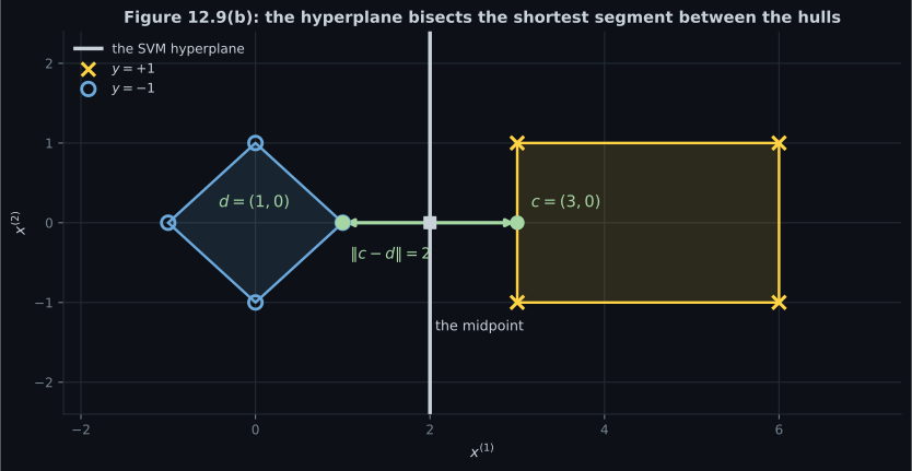
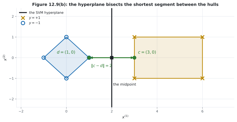
||c - d|| : 2.0000000000

The closest point of the positive hull is the midpoint of the segment joining $(3,1)$ and $(3,-1)$ — an interior point of an edge, not a vertex — while the closest point of the negative hull is the vertex $(1,0)$. The two hulls are exactly $2$ apart.

figure Figure 12.9(b): the hyperplane bisects the shortest segment between the hulls matplotlib

The SVM hyperplane is the perpendicular bisector of the shortest segment between the hulls. That is the entire geometric content of Section 12.3.2 — and it never mentions a Lagrange multiplier.

The conversion the book does not write down

§12.3.2 says the resulting problem “can be shown to be the same as that of the dual hard margin SVM” and cites Bennett and Bredensteiner. It does not say how to get from $\mathbf{c}$ and $\mathbf{d}$ to the classifier — and the vectors are not the same:

	value	norm
the hull vector $\mathbf{c} - \mathbf{d}$	$(2, 0)$	$2$
the SVM weights $\mathbf{w}^*$	$(1, 0)$	$1$

The two differ by a factor that depends on the separation. Since the hyperplane must bisect the segment perpendicularly, and must give $\pm 1$ at $\mathbf{c}$ and $\mathbf{d}$:

$$\mathbf{w}^* = \frac{2(\mathbf{c}-\mathbf{d})}{\lVert\mathbf{c}-\mathbf{d}\rVert^2}, \qquad b^* = -\Big\langle \mathbf{w}^*,\ \frac{\mathbf{c}+\mathbf{d}}{2}\Big\rangle, \qquad r = \frac{\lVert\mathbf{c}-\mathbf{d}\rVert}{2}$$

text

2(c-d)/||c-d||^2 : [1.e+00 8.e-10]
-<w, (c+d)/2>    : -2.0000000000
gap to (w*, b*)  : 8.256e-10
margin ||c-d||/2 : 1.0000000000
margin 1/||w*||  : 1.0000000000

Checked against a primal solve on $200$ random separable datasets in $2$ to $4$ dimensions:

quantity	worst disagreement
$\lVert\mathbf{w}_{\text{from hull}} - \mathbf{w}_{\text{primal}}\rVert$	$9.185\times10^{-8}$
$\lvert b_{\text{from hull}} - b_{\text{primal}}\rvert$	$4.282\times10^{-8}$
$\big\lvert \tfrac12\lVert\mathbf{c}-\mathbf{d}\rVert - r \big\rvert$	$5.051\times10^{-11}$

The margin is half the distance between the hulls. That is the cleanest one-line statement of what an SVM computes, and it appears nowhere in the chapter.

The hull weights are page 1206’s multipliers, rescaled

same_numbers.py

a = dual(X, Y, BIG)                       # page 1206's multipliers
sp, sn = a[Y > 0].sum(), a[Y < 0].sum()
print(f"mass on the positives : {sp:.10f}")
print(f"mass on the negatives : {sn:.10f}")
print(f"alpha+ / sum : {np.round(a[Y > 0] / sp, 8)}   vs a+ : {np.round(ap, 8)}")
print(f"alpha- / sum : {np.round(a[Y < 0] / sn, 8)}   vs a- : {np.round(an, 8)}")

text

mass on the positives : 0.4999999704
mass on the negatives : 0.4999999704
alpha+ / sum : [0.50000006 0.49999994 0. 0.]   vs a+ : [0.5 0.5 0.  0. ]
alpha- / sum : [1. 0. 0. 0.]   vs a- : [1. 0. 0. 0.]

Worst gap $5.780\times10^{-8}$. So the two derivations produce the same numbers up to a single rescaling: each class carries dual mass $\lVert\mathbf{w}\rVert^2/2$, and dividing by that turns Lagrange multipliers into hull weights. Equation 12.50 is not a coincidence — it is Equation 12.49 with the class masses equal.

Why the masses are equal, which is the same fact twice

Page 1206 measured $\sum_n\alpha_n = \lVert\mathbf{w}\rVert^2$; here each class carries exactly half of it, to $8.327\times10^{-16}$. That is precisely $\sum_n y_n\alpha_n = 0$ rearranged.

Read from the hull side it is obvious: each hull’s weights must sum to one because a convex combination is an average. Read from the Lagrangian side it is the derivative in $b$ set to zero. The two arguments have nothing in common and reach the same equation.

The reduced hull

The section ends with a remark rather than a derivation:

To obtain the soft margin dual, we consider the reduced hull. The reduced hull is similar to the convex hull but has an upper bound to the size of the coefficients $\alpha$. The maximum possible value of the elements of $\alpha$ restricts the size that the convex hull can take.

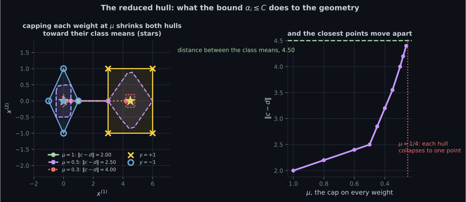
Capping every weight at $\mu$ and re-solving:

text

      mu                  c                  d    ||c-d||    margin
    1.00            [3. 0.]          [ 1. -0.]   2.000000  1.000000
    0.60            [3. 0.]        [ 0.6 -0. ]   2.400000  1.200000
    0.50          [ 3. -0.]          [0.5 0. ]   2.500000  1.250000
    0.40        [ 3.6 -0. ]          [0.4 0. ]   3.200000  1.600000
    0.34        [3.96 0.  ]      [ 0.34 -0.  ]   3.620000  1.810000
    0.30          [4.2 0. ]        [ 0.2 -0. ]   4.000000  2.000000
    0.26      [ 4.44 -0.  ]      [ 0.04 -0.  ]   4.400000  2.200000

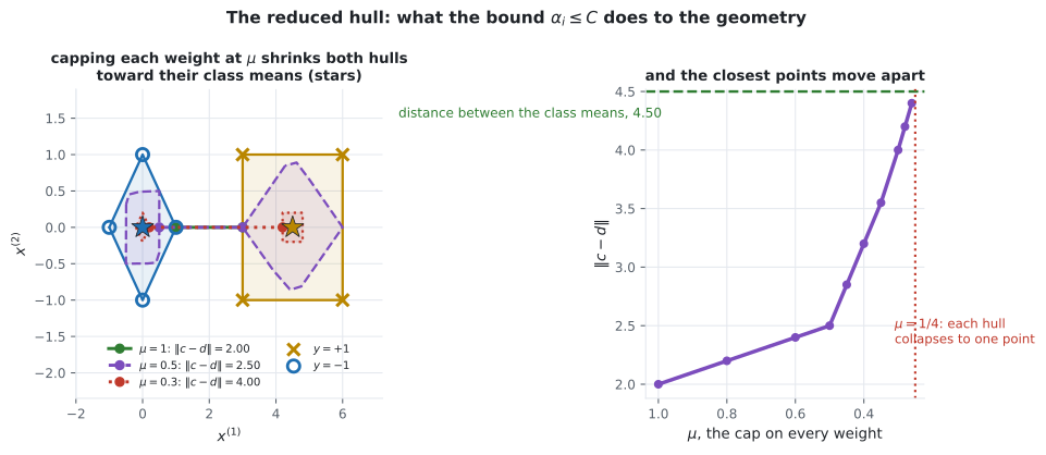
Each hull contracts toward its own class mean, and the two closest points move apart. With four points per class, $\mu = \tfrac14$ forces every weight to exactly $\tfrac14$ — each hull collapses to a single point, the class mean, and the “closest pair” is the pair of means, $4.5$ apart:

text

the positive class mean : [4.5 0.]
the negative class mean : [0.  0.]
their distance          : 4.500000

Below $\mu = \tfrac14$ the constraint $\sum_n\alpha_n = 1$ cannot be satisfied at all, so the reduced hull is empty. The bound $\mu$ is doing exactly what $C$ did on page 1204: a looser cap means the model can commit its weight to a few extreme examples, a tighter cap forces it to spread weight and average toward the class centre.

figure The reduced hull: what the bound alpha_i <= C does to the geometry matplotlib

Read the right panel right-to-left as the cap tightens. At μ = 1/4 each hull has collapsed to its class mean and the SVM has become a nearest-class-mean classifier — the same degeneration page 1204 measured as C going to zero.

The correspondence is structural, not numerical

It is tempting to read off a formula relating $\mu$ to $C$ from these two tables. Resist it. The soft-margin dual constrains $\alpha_n \leq C$ with $\sum_n\alpha_n$ free; the reduced hull constrains $\alpha_n \leq \mu$ with each class’s weights summing to $1$. The two are related by the class mass $S = \lVert\mathbf{w}\rVert^2/2$, which is itself an output of the solve — so $\mu = C/S$ holds only once you already know the answer.

What transfers without arithmetic is the shape of the trade: a tighter cap spreads the weight, contracts the hulls, and moves the decision boundary toward the line bisecting the class means.

pch.quizTag Check your understanding

1. A From differentiating the Lagrangian in b B From requiring each hull's weights to sum to one: the positive weights sum to 1 and the negative weights sum to 1, and their signed difference is 1 - 1 = 0 C From the box constraint D From the representer theorem
   pch.quizShowAnswer

   B — From requiring each hull's weights to sum to one: the positive weights sum to 1 and the negative weights sum to 1, and their signed difference is 1 - 1 = 0

2. A They are equal; the difference is a solver artefact B w* is the unit vector in the direction of c - d C w* = 2(c - d)/||c - d||^2, and the margin is half the distance between the hulls — verified across 200 datasets to 9.2e-08 D w* = (c - d)/2
   pch.quizShowAnswer

   C — w* = 2(c - d)/||c - d||^2, and the margin is half the distance between the hulls — verified across 200 datasets to 9.2e-08

3. A They are unrelated quantities B The hull weights are the multipliers divided by their own class's total mass, which is half the squared norm of w — measured to agree within 5.8e-08 C The hull weights are twice the multipliers D The multipliers are the hull weights squared
   pch.quizShowAnswer

   B — The hull weights are the multipliers divided by their own class's total mass, which is half the squared norm of w — measured to agree within 5.8e-08

4. A The hulls grow and the closest points converge B Nothing until mu reaches zero C Each hull contracts toward its class mean and the closest points move apart, from 2.00 to 4.40; at mu = 1/4 each hull is a single point and the classifier bisects the class means D The problem becomes infeasible immediately
   pch.quizShowAnswer

   C — Each hull contracts toward its class mean and the closest points move apart, from 2.00 to 4.40; at mu = 1/4 each hull is a single point and the classifier bisects the class means

Exercises

Exercise 1 – Find the two closest points of the hulls

pch.exerciseTag pch.exerciseTitle

Exercise 2 – Convert the segment into a classifier

pch.exerciseTag pch.exerciseTitle

Exercise 3 – Shrink the hulls and watch them separate

pch.exerciseTag pch.exerciseTitle

Recall card

• Section 12.3.2 reaches the dual by a route with no calculus in it: wrap each class in its convex hull and find the two closest points.
• The convex hull is every weighted average with non-negative weights summing to one, so requiring that sum on each class and taking the signed difference gives the dual’s equality constraint directly.
• On the running example the closest points are (3, 0) and (1, 0), exactly two apart. The positive one is inside an edge rather than at a vertex — it is the average of the two support vectors.
• The SVM hyperplane is the perpendicular bisector of that segment. That is the whole geometric content of the section.
• The book does not say how to convert the segment into a classifier. The weight vector is twice the segment divided by its squared length, and the intercept is minus the inner product of that with the segment’s midpoint.
• Checked on 200 random datasets, the conversion agrees with a primal solve to 9.2e-08 in w and 4.3e-08 in b.
• The margin is half the distance between the two hulls — the shortest true statement of what an SVM computes, and one the chapter never makes.
• The hull weights are the Lagrange multipliers renormalised per class. Each class carries dual mass equal to half the squared norm of w, and dividing by it turns one into the other, to 5.8e-08.
• So the two derivations are the same numbers up to a single rescaling, reached by arguments that have nothing in common.
• The reduced hull is the soft margin’s geometry. Capping every weight contracts each hull toward its class mean and pushes the closest points apart, from 2.00 to 4.40 on this data.
• At a cap of one over the class size each hull collapses to a single point and the classifier bisects the class means — the same degeneration page 1204 measured as C goes to zero.
• But the correspondence between the cap and C is structural, not numerical: relating them needs the class mass, which is an output of the solve rather than an input.

Next: Kernels — §12.4, where the inner product in Equation 12.41 is replaced by something else and the whole chapter stops being linear.