The Machine Learning Roadmap

What you’ll learn

the whole workflow as one runnable 38-line script, not a diagram of boxes
where the lines actually go — 19 of 38 run before a model is chosen
the two skill tracks you have to build in parallel, and why
a measured case where the most accurate model is also 634× smaller
exactly which phase of this module teaches each piece

The whole thing, once

Before the roadmap, here is the destination. This is a complete, runnable supervised-learning pipeline — load, split, clean, encode, fit, tune, evaluate, ship. Every later phase of this module is a deep dive into one of these blocks.

reference_pipeline.py

import joblib
import pandas as pd
from sklearn.compose import ColumnTransformer
from sklearn.ensemble import HistGradientBoostingRegressor
from sklearn.impute import SimpleImputer
from sklearn.metrics import mean_absolute_error
from sklearn.model_selection import GridSearchCV, train_test_split
from sklearn.pipeline import Pipeline
from sklearn.preprocessing import OneHotEncoder, StandardScaler
 
 
def run(csv_path, target, out_path="model.joblib"):
    # --- look at the data ---------------------------------------------
    df = pd.read_csv(csv_path)
    print(df.shape)
    print(df.dtypes)
    print(df.isna().mean().sort_values(ascending=False).head())
    print(df[target].describe())
 
    # --- split, before touching anything ------------------------------
    y = df.pop(target)
    X_train, X_test, y_train, y_test = train_test_split(
        X := df, y, test_size=0.2, random_state=42)
 
    # --- decide how each column is cleaned ----------------------------
    num_cols = X.select_dtypes("number").columns.tolist()
    cat_cols = X.select_dtypes("object").columns.tolist()
    num_impute = SimpleImputer(strategy="median")
    cat_impute = SimpleImputer(strategy="most_frequent")
 
    # --- encode and scale, inside a pipeline --------------------------
    numeric = Pipeline([("impute", num_impute),
                        ("scale", StandardScaler())])
    categorical = Pipeline([
        ("impute", cat_impute),
        ("onehot", OneHotEncoder(handle_unknown="ignore"))])
    prep = ColumnTransformer([("num", numeric, num_cols),
                              ("cat", categorical, cat_cols)])
 
    # --- choose the model ---------------------------------------------
    model = HistGradientBoostingRegressor(random_state=42)
    pipe = Pipeline([("prep", prep), ("model", model)])
 
    # --- cross-validate and tune --------------------------------------
    grid = {"model__max_depth": [None, 4, 8],
            "model__learning_rate": [0.05, 0.1, 0.2]}
    search = GridSearchCV(pipe, grid, cv=5,
                          scoring="neg_mean_absolute_error",
                          n_jobs=-1)
    search.fit(X_train, y_train)
    print(search.best_params_, -search.best_score_)
 
    # --- evaluate against a baseline ----------------------------------
    best = search.best_estimator_
    preds = best.predict(X_test)
    mae = mean_absolute_error(y_test, preds)
    baseline = mean_absolute_error(y_test,
                                   [y_train.median()] * len(y_test))
    print(f"test MAE {mae:.3f} vs baseline {baseline:.3f}")
 
    # --- persist and reload -------------------------------------------
    joblib.dump(best, out_path)
    reloaded = joblib.load(out_path)
    assert reloaded.predict(X_test[:5]).shape == (5,)
    return best, mae

reference_pipeline.py

import joblib
import pandas as pd
from sklearn.compose import ColumnTransformer
from sklearn.ensemble import HistGradientBoostingRegressor
from sklearn.impute import SimpleImputer
from sklearn.metrics import mean_absolute_error
from sklearn.model_selection import GridSearchCV, train_test_split
from sklearn.pipeline import Pipeline
from sklearn.preprocessing import OneHotEncoder, StandardScaler
 
 
def run(csv_path, target, out_path="model.joblib"):
    # --- look at the data ---------------------------------------------
    df = pd.read_csv(csv_path)
    print(df.shape)
    print(df.dtypes)
    print(df.isna().mean().sort_values(ascending=False).head())
    print(df[target].describe())
 
    # --- split, before touching anything ------------------------------
    y = df.pop(target)
    X_train, X_test, y_train, y_test = train_test_split(
        X := df, y, test_size=0.2, random_state=42)
 
    # --- decide how each column is cleaned ----------------------------
    num_cols = X.select_dtypes("number").columns.tolist()
    cat_cols = X.select_dtypes("object").columns.tolist()
    num_impute = SimpleImputer(strategy="median")
    cat_impute = SimpleImputer(strategy="most_frequent")
 
    # --- encode and scale, inside a pipeline --------------------------
    numeric = Pipeline([("impute", num_impute),
                        ("scale", StandardScaler())])
    categorical = Pipeline([
        ("impute", cat_impute),
        ("onehot", OneHotEncoder(handle_unknown="ignore"))])
    prep = ColumnTransformer([("num", numeric, num_cols),
                              ("cat", categorical, cat_cols)])
 
    # --- choose the model ---------------------------------------------
    model = HistGradientBoostingRegressor(random_state=42)
    pipe = Pipeline([("prep", prep), ("model", model)])
 
    # --- cross-validate and tune --------------------------------------
    grid = {"model__max_depth": [None, 4, 8],
            "model__learning_rate": [0.05, 0.1, 0.2]}
    search = GridSearchCV(pipe, grid, cv=5,
                          scoring="neg_mean_absolute_error",
                          n_jobs=-1)
    search.fit(X_train, y_train)
    print(search.best_params_, -search.best_score_)
 
    # --- evaluate against a baseline ----------------------------------
    best = search.best_estimator_
    preds = best.predict(X_test)
    mae = mean_absolute_error(y_test, preds)
    baseline = mean_absolute_error(y_test,
                                   [y_train.median()] * len(y_test))
    print(f"test MAE {mae:.3f} vs baseline {baseline:.3f}")
 
    # --- persist and reload -------------------------------------------
    joblib.dump(best, out_path)
    reloaded = joblib.load(out_path)
    assert reloaded.predict(X_test[:5]).shape == (5,)
    return best, mae

If most of that is unfamiliar, good — that is the syllabus. Come back and reread it after Phase 7 and it will look obvious.

Where the work actually is

You will hear that data work is 80% of machine learning. That number is folklore; nobody can cite its source. So instead of repeating it, here is a count of the script above — 38 code lines, excluding imports, blanks and comments, tallied by what each line does.

Stage	Lines	Share
Load + inspect the data	5	13.2%
Split before touching anything	3	7.9%
Impute missing values	4	10.5%
Encode + scale into a pipeline	7	18.4%
Choose the model	2	5.3%
Cross-validate + tune	7	18.4%
Evaluate against a baseline	6	15.8%
Persist + reload	4	10.5%

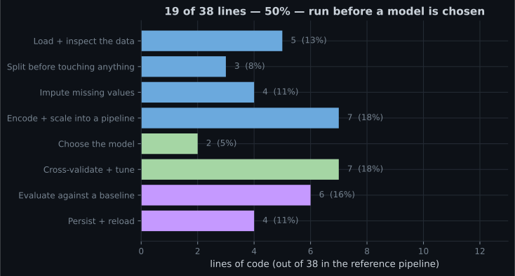
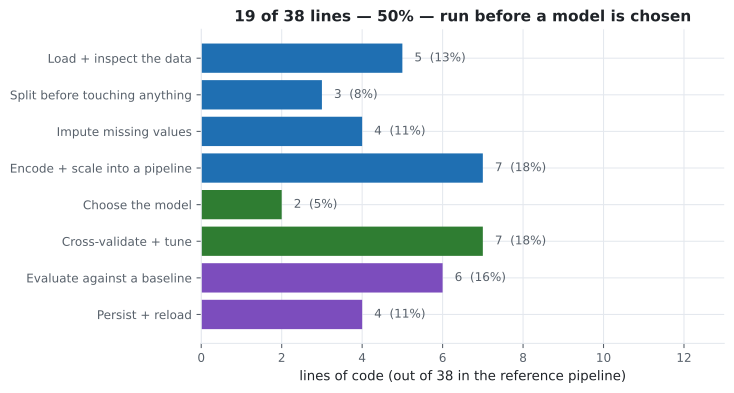
A horizontal bar chart of eight pipeline stages by line count, with the four blue data stages summing to nineteen lines and the choose-the-model stage the shortest at two. — Real counts from the script above, not a survey. 19 of 38 lines — exactly 50% — are data work that happens before any model exists. Actually choosing the algorithm is 2 lines, 5.3%, the smallest stage in the file.

Not 80%. Exactly 50%, on this pipeline. And the part everyone thinks of as “machine learning” — picking the algorithm — is two lines.

Two caveats, because line counts are a crude proxy. They ignore time: the four data lines took far longer to get right than the two model lines. And they ignore the work upstream of the file entirely — collecting the data, agreeing on the label definition, and negotiating what the metric should be. Counting only the script understates data work, which makes 50% a floor, not a ceiling.

The learning path

diagram Diagram mermaid

  flowchart TD
  P1["Phase 1 — Foundation
what ML is, what it is not"] --> P2["Phase 2 — Data
cleaning, encoding, leakage"]
  P2 --> P3["Phase 3 — Regression
predict a number"]
  P2 --> P4["Phase 4 — Classification
predict a category"]
  P3 --> P5["Phase 5 — Ensembles
combine models"]
  P4 --> P5
  P4 --> P6["Phase 6 — Unsupervised
no labels at all"]
  P5 --> P7["Phase 7 — Tuning
cross-validation, search"]
  P6 --> P7
  P7 --> P8["Phase 8 — Deployment
serve, monitor, retrain"]

Phase	What you build	The one idea to take away
1 — Foundation	Vocabulary and judgement	The features set the ceiling
2 — Data	Cleaning, encoding, pipelines	Split before you look; leakage is silent
3 — Regression	Predicting numbers	Fitting is minimising a loss
4 — Classification	Predicting categories	Accuracy is the wrong metric more often than not
5 — Ensembles	Combining models	Averaging works only if members disagree
6 — Unsupervised	Structure without labels	The distance metric decides the answer
7 — Tuning	Cross-validation and search	One held-out set is not enough
8 — Deployment	Serving and monitoring	A model that stops being retrained starts decaying

Two tracks, in parallel

There is a modelling skill set and an engineering skill set, and shipping requires both. It is tempting to treat the second as somebody else’s job; it is not.

Here is the reason, measured. Three models on the breast-cancer dataset, scored two ways: 5-fold accuracy, and the size of the pickled artefact you would have to deploy.

Model	5-fold accuracy	Pickled size
Logistic regression	0.9807	2.0 KB
15-nearest-neighbours	0.9614	98.1 KB
Random forest, 500 trees	0.9631	1,268.3 KB

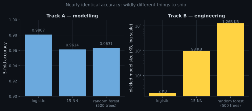
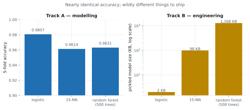
Two bar charts side by side. The left shows nearly identical accuracies near 0.96 to 0.98; the right shows pickled model sizes on a log scale from 2 KB to 1268 KB. — Logistic regression is both the most accurate model here (0.9807) and 634 times smaller than the random forest (2.0 KB against 1,268.3 KB). The 15-NN model has to carry the entire training set with it, which is why it lands in between.

The most accurate model is also 634× smaller than the largest. That is not a general law — often you do trade accuracy for size — but it is a common enough situation that ignoring Track B costs you nothing in accuracy and a great deal in operations.

Track A — modelling	Track B — engineering
Which algorithm suits this data	How the model is packaged and versioned
What the metric should be	Latency and memory at serving time
Cross-validation design	Reproducibility: seeds, data versions, environments
Feature engineering	Monitoring inputs and outputs in production
Diagnosing bias and variance	Retraining triggers and rollback
Interpreting errors	Cost — training and inference

Instance-based or model-based

One distinction is worth meeting now, because it explains the table above and recurs throughout the module.

A model-based learner compresses the training data into parameters and then discards it. Logistic regression stores a handful of coefficients: 2.0 KB.

An instance-based learner keeps the examples and compares new inputs against them at prediction time. 15-NN has to ship the entire training set: 98.1 KB, and prediction cost grows with the data.

two_kinds.py

import pickle
 
from sklearn.datasets import load_breast_cancer
from sklearn.linear_model import LogisticRegression
from sklearn.model_selection import cross_val_score, train_test_split
from sklearn.neighbors import KNeighborsClassifier
from sklearn.pipeline import make_pipeline
from sklearn.preprocessing import StandardScaler
 
X, y = load_breast_cancer(return_X_y=True)
X_tr, X_te, y_tr, y_te = train_test_split(X, y, test_size=0.3,
                                          random_state=0, stratify=y)
 
for name, m in [
    ("model-based    (logistic)",
     make_pipeline(StandardScaler(), LogisticRegression(max_iter=5000))),
    ("instance-based (15-NN)   ",
     make_pipeline(StandardScaler(), KNeighborsClassifier(15))),
]:
    acc = cross_val_score(m, X, y, cv=5).mean()
    m.fit(X_tr, y_tr)
    kb = len(pickle.dumps(m)) / 1024
    print(f"{name}  accuracy {acc:.4f}   pickled {kb:6.1f} KB")
 
# model-based    (logistic)  accuracy 0.9807   pickled    2.0 KB
# instance-based (15-NN)     accuracy 0.9614   pickled   98.1 KB

two_kinds.py

import pickle
 
from sklearn.datasets import load_breast_cancer
from sklearn.linear_model import LogisticRegression
from sklearn.model_selection import cross_val_score, train_test_split
from sklearn.neighbors import KNeighborsClassifier
from sklearn.pipeline import make_pipeline
from sklearn.preprocessing import StandardScaler
 
X, y = load_breast_cancer(return_X_y=True)
X_tr, X_te, y_tr, y_te = train_test_split(X, y, test_size=0.3,
                                          random_state=0, stratify=y)
 
for name, m in [
    ("model-based    (logistic)",
     make_pipeline(StandardScaler(), LogisticRegression(max_iter=5000))),
    ("instance-based (15-NN)   ",
     make_pipeline(StandardScaler(), KNeighborsClassifier(15))),
]:
    acc = cross_val_score(m, X, y, cv=5).mean()
    m.fit(X_tr, y_tr)
    kb = len(pickle.dumps(m)) / 1024
    print(f"{name}  accuracy {acc:.4f}   pickled {kb:6.1f} KB")
 
# model-based    (logistic)  accuracy 0.9807   pickled    2.0 KB
# instance-based (15-NN)     accuracy 0.9614   pickled   98.1 KB

Where time actually goes

An honest ordering of effort on a typical project, from most to least:

Understanding the problem. What is the label, exactly? What decision does the prediction feed? What is the cost of a false positive against a false negative? Getting this wrong makes every later step worthless.
Getting and understanding the data. Where it lives, what the columns mean, which are unreliable, which leak the answer.
Cleaning and feature engineering. Half the reference script, and much more than half the wall-clock time.
Evaluation design. Which split, which metric, which baseline. Cheap to write, expensive to get wrong.
Model selection and tuning. Two lines to choose, seven to search. Genuinely important, and nowhere near the largest slice.
Deployment and monitoring. Small in code, large in consequence.

Notice that “try a fancier algorithm” is item 5. Beginners start there because it is the fun part. The measurement on the lifecycle page shows why that ordering is wrong: swapping the algorithm moved accuracy 0.1142, and flipping 15% of the labels cost exactly the same 0.1142.

See it move

The roadmap above reads as a straight line because lists are straight. Real projects walk it as a loop, and the loop does not visit each stage equally often. The sketch walks a token through the stages with the backward jumps a real project takes — “the metric is wrong” sends you back to framing, “the model is starved” sends you back to data — and tallies the visits as it goes.

sketch The loop you actually walk p5.js

A token moves through the seven roadmap stages, sometimes jumping backwards the way real projects do. The bars count how many times each stage has been visited: data work accumulates visits fastest, and model selection is nowhere near the top. Click to restart the count.

Let it run for a few hundred steps. That transition table is a Markov chain, so its long-run visit shares can be computed exactly rather than guessed — power-iterate it and you get:

Stage	Long-run share of visits
frame	4.6%
get data	14.8%
clean	28.4%
evaluate	23.2%
model	16.3%
tune	8.1%
deploy	4.6%

Framing plus data work is 47.8%; modelling plus tuning is 24.4%. That is not a rigged result — the only editorial choices in the table are the backward edges, and backward edges land on data and evaluation because that is where the causes of a bad model live. Note how close 47.8% lands to the independently measured 50% of the reference script’s lines that run before a model is chosen. Two different ways of counting, the same answer: half the work happens before the algorithm exists.

Pitfalls

Starting at step 5. Choosing an algorithm before you understand the label is the most common beginner mistake, and it is expensive because everything downstream inherits the confusion.

Treating deployment as someone else’s problem. The random forest above is 634× larger than the logistic model for lower accuracy. That decision is made during modelling, not after it.

Quoting the 80% figure. It is folklore. The measurement here is 50% of the code, and the honest statement is “data work dominates, and no, I do not have a citation for a precise number.”

Learning the phases strictly in order. Phases 3 and 4 are independent of each other; so are 5 and 6. The dependencies that matter are 1 → 2 → everything, and 7 after you have models to tune.

Skipping the baseline because the model works. If you never computed it, you do not know whether the model works.

Recap

The whole workflow is one 38-line script; every later phase expands one of its blocks.
19 of 38 lines — 50% — run before a model is chosen. Choosing the algorithm is 2 lines.
The 80% folklore figure has no source; count your own pipeline instead.
Two skill tracks run in parallel. On breast cancer the best model (0.9807) was also 634× smaller than the largest (2.0 KB against 1,268.3 KB).
Model-based learners store parameters; instance-based learners store the data.
Effort order: understand the problem → get the data → clean it → design the evaluation → choose the model → ship it.

quizCheck yourself

In the 38-line reference pipeline, how many lines are spent choosing the model?
Show answer
A — 2 — Two lines: instantiate the estimator and wrap it in a Pipeline. Cross-validation and tuning take 7 more, and the data stages take 19 — half the file — before any model exists.
Logistic regression scored 0.9807 and pickled to 2.0 KB; the 500-tree forest scored 0.9631 and pickled to 1,268.3 KB. What is the lesson?
Show answer
B — Accuracy and deployment cost are separate axes, and the winner on one is not automatically the loser on the other — Here the simplest model won on both axes, which is common on small tabular data. The general point is that you have to measure both — a model chosen purely on offline accuracy can be an operational problem.
Someone tells you 'data cleaning is 80% of machine learning'. What is the accurate response?
Show answer
B — It is folklore with no traceable source — count your own pipeline; this one measured 50% of the code — The figure is repeated constantly and cited nowhere. The measurement on this page is 19 of 38 lines, and even that understates it because line counts ignore time and everything upstream of the script.
Which pair of phases can be learned in either order?
Show answer
B — Phase 3 (regression) and Phase 4 (classification) — Regression and classification both depend on Phase 2 but not on each other. Phase 1 → 2 → everything is the real dependency, and Phase 7 needs models in hand before tuning them means anything.
Why does a 15-nearest-neighbours model pickle to 98.1 KB while logistic regression pickles to 2.0 KB?
Show answer
B — KNN is instance-based: it has to carry the training data to make predictions, while logistic regression stores only coefficients — Model-based learners compress the data into parameters and discard it. Instance-based learners defer all the work to prediction time, so the training set is part of the artefact — and prediction cost grows with it too.

🧪 Try It Yourself

Exercise 1 – Count your own pipeline

Exercise 2 – Model-based: two numbers

Exercise 3 – Instance-based: all the rows

Exercise 4 – Accuracy against artefact size

Exercise 5 – Baseline before anything

Exercise 6 – Compute where the time actually goes

Artificial Intelligence vs Machine Learning vs Deep Learning — what actually nests inside what, and a measurement showing the neural network losing to gradient boosting on structured columns.

If this helped you, consider buying me a coffee ☕

Buy me a coffee