Transfer Learning - Using Pre-trained Models

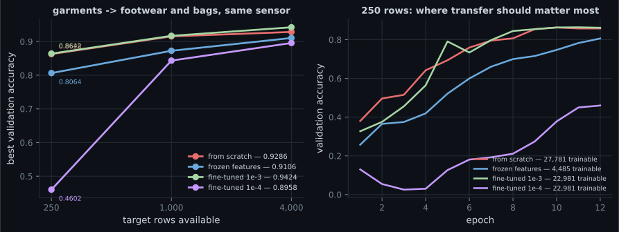
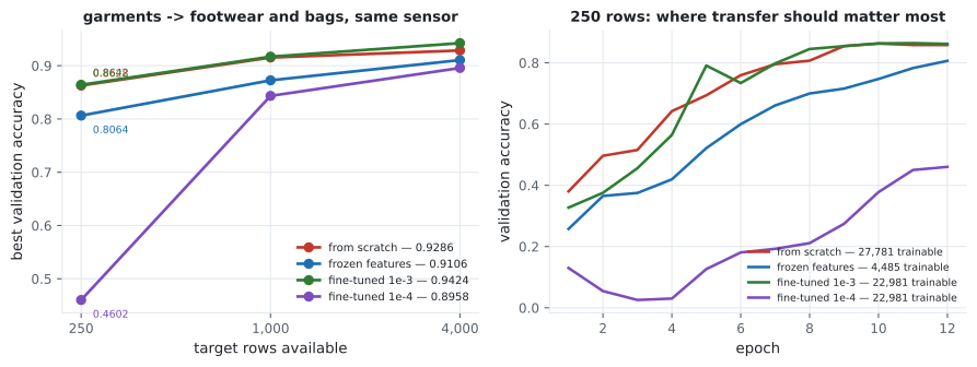
Transfer learning is usually sold as free accuracy: take a model somebody else trained, reuse its features, win. This page builds the setup properly — a source task and a target task from the same sensor with disjoint labels — and measures four strategies against training from scratch.

The honest headline is that transfer bought almost nothing here, and the reasons why are more useful than another demonstration that it works.

Target rows	From scratch	Frozen features	Fine-tuned 1e-3	Fine-tuned 1e-4
250	0.8628	0.8064 (−0.0564)	0.8642 (+0.0014)	0.4602 (−0.4026)
1,000	0.9154	0.8726 (−0.0428)	0.9170 (+0.0016)	0.8434 (−0.0720)
4,000	0.9286	0.9106 (−0.0180)	0.9424 (+0.0138)	0.8958 (−0.0328)

Fine-tuning won by 0.0014 where transfer is supposed to matter most. Freezing the backbone lost at every size. And the only large number in the table is the damage done by one wrong hyperparameter.

The setup

Nothing is downloaded. The backbone is pre-trained here, on a task that is genuinely different from the target:

	Classes	Rows	Source accuracy
source (related)	t-shirt, pullover, dress, coat, shirt	12,000	0.7114
source (unrelated)	MNIST handwritten digits	12,000	0.9240
target	trouser, sandal, sneaker, bag, boot	250 – 4,000	—

The related split is the fair version of the experiment: same 28×28 greyscale sensor, same preprocessing, no shared labels. A backbone trained to tell a coat from a shirt has never seen a shoe.

What you’ll learn

• The four strategies, and what each one actually trains: 4,485 parameters frozen against 27,781 from scratch.
• Why layer.trainable = False does nothing until you recompile.
• The learning-rate trap that cost 0.4026 accuracy — and why it is a fair comparison only when the rate is held constant.
• A linear probe, the cleanest way to ask what a backbone actually learned.
• Why the unrelated source scored 0.9124 against the related source’s 0.9170 — nearly the same — and what that says about fine-tuning.
• The conditions under which transfer learning earns its reputation, none of which hold here.

The four strategies

Freeze, or fine-tune, or start over

backbone = pretrained_backbone()             # three conv blocks, 23,296 params
 
for layer in backbone.layers:                # 1. frozen features
    layer.trainable = False
 
for layer in backbone.layers:                # 2. fine-tune the top block
    layer.trainable = layer.name.startswith("block2_")
 
model = keras.Model(backbone.input, head(backbone.output))
model.compile(keras.optimizers.Adam(1e-3), ...)   # <- the freeze takes effect HERE

trainable is read at compile time. Flip it afterwards and the already-built training function keeps updating the weights you thought you had frozen — Exercise 3 measures exactly that, and it is silent.

figure Garments to footwear and bags, same sensor, disjoint labels matplotlib

Three of the four curves are on top of each other, which is the result: at 250 target rows, training from scratch reaches 0.8628 and the best transfer strategy reaches 0.8642. The outlier is the low learning rate, and the right panel shows why — at 1e-4 the model is simply still training at epoch 12. That is not a property of fine-tuning, it is a budget mismatch, and it is the most common way transfer-learning comparisons get rigged.

Why transfer bought so little

Three conditions have to hold before a pre-trained backbone helps, and none of them do here.

1. The source model must be better than what you can train yourself. This backbone is 23,296 parameters trained on 12,000 rows to 0.7114 accuracy. ImageNet backbones are 10⁷–10⁸ parameters trained on 10⁶ images. There is no knowledge advantage to transfer.
2. The target task must be hard enough that data is the binding constraint. Telling a trouser from a sneaker from a bag is easy: from scratch reaches 0.8628 with 250 examples. There is no gap for a backbone to close.
3. The domains must differ in the right way. The source and target are the same sensor, same resolution, same statistics — so the low-level features a fresh model learns in two epochs are the same ones the backbone offers.

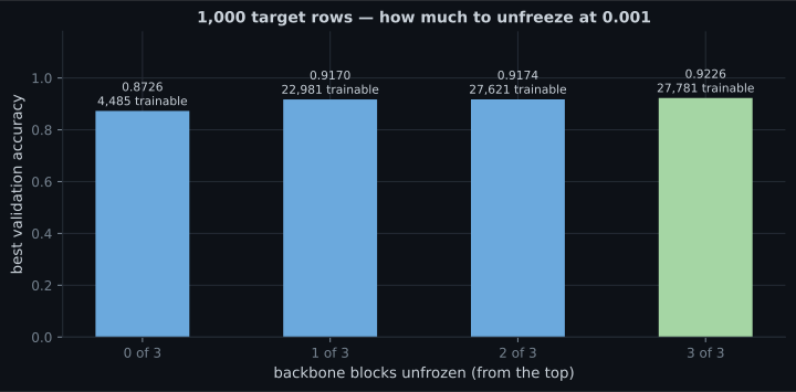
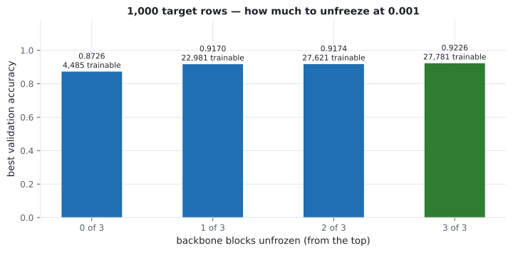
The fourth column of the unfreeze sweep makes the point precisely:

Blocks unfrozen	Trainable parameters	Best validation accuracy
0 (frozen features)	4,485	0.8726
1	22,981	0.9170
2	27,621	0.9174
3 (all — nothing frozen)	27,781	0.9226

figure 1,000 target rows — how much to unfreeze matplotlib

Accuracy increases monotonically with how much of the backbone you let move, and the best result is the one that keeps nothing frozen. On a task where the pre-trained features are not better than freshly learned ones, freezing is a pure constraint — the usual advice to freeze first exists for the opposite regime, where the backbone is strong and the target data is too small to fine-tune safely without destroying it.

The source task mattered less than expected

Source	Frozen features	Fine-tuned 1e-3
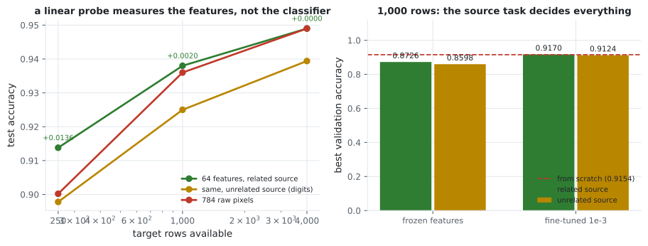
related (garments)	0.8726	0.9170
unrelated (MNIST digits)	0.8598	0.9124

A backbone trained on handwritten digits transferred to footwear almost as well as one trained on clothing — 0.9124 against 0.9170. Frozen, the gap is larger (0.8598 against 0.8726), which is the expected direction: when the features cannot move, their relevance matters. Once fine-tuning is allowed to rewrite them at 1e-3, the initialisation is mostly forgotten.

This is worth stating plainly because it cuts against the usual advice. “Choose a source task close to your target” is sound, but its effect here was 0.0046 — an order of magnitude smaller than the effect of choosing the learning rate correctly.

The linear probe

The cleanest question you can ask a backbone is: how good are your features, ignoring the classifier? Freeze everything, extract the 64-dimensional pooled vector, and fit plain logistic regression to it — then do the same with the 784 raw pixels.

Target rows	On 64 related features	On 64 unrelated features	On 784 raw pixels
250	0.9138	0.8978	0.9002
1,000	0.9380	0.9250	0.9360
4,000	0.9490	0.9394	0.9490

figure A linear probe measures the features, not the classifier matplotlib

At 250 rows the pre-trained features beat raw pixels by 0.0136 — a 64-number summary outperforming 784 pixels is a real compression win. By 4,000 rows the advantage is exactly 0.0000: given enough data, a linear model on raw pixels does just as well. That convergence is the whole shape of transfer learning in one chart, and it is why the technique is described as a small-data method.

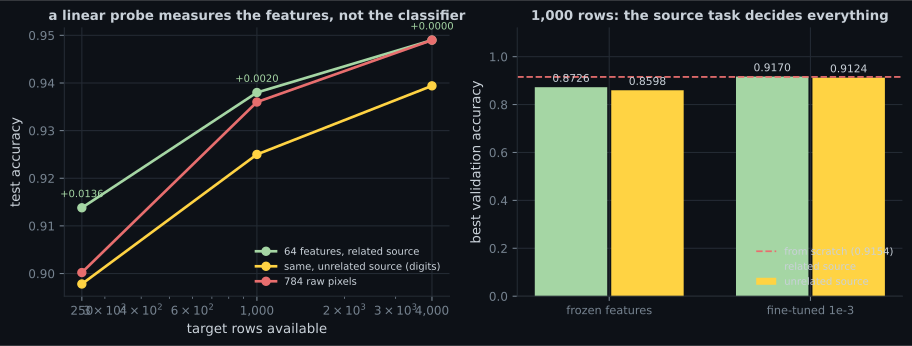
The probe result is the most positive number on this page, and it is also the smallest one that matters: 64 numbers, from a network that never saw a shoe, carry as much linearly-separable information as 784 raw pixels — and slightly more when data is scarce.

diagram Diagram mermaid

  flowchart TB
  A["is your target data small
relative to the task's difficulty?"] -->|"no"| B["train from scratch
— 0.9286 here at 4,000 rows"]
  A -->|"yes"| C["is the source model much stronger
than anything you can train?"]
  C -->|"no"| D["transfer buys ~0
— +0.0014 measured"]
  C -->|"yes"| E["fine-tune, same learning rate
as your scratch baseline"]
  E --> F{"target data tiny
or very different?"}
  F -->|"yes"| G["freeze the lower blocks first"]
  F -->|"no"| H["unfreeze everything
— best result here, 0.9226"]

sketch Freeze, fine-tune, or start over p5.js Pause Restart

Click blocks to freeze or unfreeze them and see the trainable-parameter count, with the measured accuracy at 1,000 target rows.

sketch The measured table, ranked p5.js Pause Restart

Click a column to rank every row by it. The bars are that column's values and the highest and lowest are computed from the numbers, not written in.

Pitfalls

• Comparing fine-tuning against scratch at different learning rates. 1e-4 scored 0.4602 against scratch’s 0.8628 at 250 rows — a 0.4026 gap that says nothing about transfer learning and everything about the budget.
• Flipping trainable after compiling. The change is ignored until you recompile, silently.
• Freezing by default. Freezing lost at all three sizes here (−0.0564, −0.0428, −0.0180), and the best unfreeze setting was “unfreeze everything”.
• Assuming a weak backbone still helps. A 23,296-parameter backbone at 0.7114 source accuracy has nothing to lend; the technique’s reputation comes from backbones three orders of magnitude larger.
• Choosing the source task carefully and the learning rate carelessly. Related vs unrelated source was worth 0.0046; the learning rate was worth 0.4026.
• Reporting transfer results without a from-scratch baseline. 0.9424 sounds excellent until scratch scores 0.9286.
• Skipping the linear probe. It separates “the features are good” from “the classifier trained well”, and it takes seconds.

Recap

• Source: five garment classes (0.7114). Target: five footwear-and-bag classes, disjoint labels, same sensor.
• Best transfer against scratch: +0.0014 at 250 rows, +0.0016 at 1,000, +0.0138 at 4,000. Freezing lost at every size.
• Fine-tuning at 1e-4 while scratch ran at 1e-3 cost 0.4026 at 250 rows — a budget artefact, not a finding.
• Unfreezing more always helped: 0.8726 → 0.9170 → 0.9174 → 0.9226.
• An unrelated source (MNIST digits) fine-tuned to 0.9124 against the related source’s 0.9170 — once the weights can move, the initialisation mostly washes out.
• A linear probe on 64 frozen features beat 784 raw pixels by 0.0136 at 250 rows and by 0.0000 at 4,000.

Next

Freezing and fine-tuning are the two ends of a spectrum, and there is a third option in between that trains under 3% of the weights: Fine-Tuning and Parameter-Efficient Tuning (LoRA).

pch.quizTag pch.quizDefaultTitle

1. Fine-tuning beat training from scratch by 0.0014 at 250 target rows. What is the most likely reason transfer bought so little?

   A The fine-tuning was implemented incorrectly B The backbone is 23,296 parameters trained to 0.7114 accuracy — it has no knowledge advantage over what a fresh model learns on the same easy target task C 250 rows is too many for transfer to help D The source and target must share labels
   pch.quizShowAnswer

   B — The backbone is 23,296 parameters trained to 0.7114 accuracy — it has no knowledge advantage over what a fresh model learns on the same easy target task — Transfer learning's reputation comes from backbones three orders of magnitude larger trained on far more data. Scale is the mechanism, not the ceremony of loading weights.

2. Fine-tuning at 1e-4 scored 0.4602 while training from scratch at 1e-3 scored 0.8628. What does that comparison establish?

   A Fine-tuning is worse than training from scratch B Nothing about transfer learning — the two runs used different learning rates, so the 0.4026 gap measures the budget, and the per-epoch curve shows the 1e-4 model still climbing at epoch 12 C The pre-trained weights were corrupted D A low learning rate always fails
   pch.quizShowAnswer

   B — Nothing about transfer learning — the two runs used different learning rates, so the 0.4026 gap measures the budget, and the per-epoch curve shows the 1e-4 model still climbing at epoch 12 — It is the same class of error as comparing augmented and un-augmented models at a fixed epoch count. Hold everything constant except the thing you are measuring.

3. Accuracy rose monotonically as more of the backbone was unfrozen: 0.8726, 0.9170, 0.9174, 0.9226. When is the usual 'freeze first' advice right?

   A Always — freezing prevents overfitting B When the backbone is genuinely stronger than anything you could train and the target data is small enough that fine-tuning would destroy its features C Only for models with batch normalisation D Never; freezing is obsolete
   pch.quizShowAnswer

   B — When the backbone is genuinely stronger than anything you could train and the target data is small enough that fine-tuning would destroy its features — Here neither condition held, so freezing was a pure constraint on capacity and cost accuracy at every dataset size.

4. A backbone pre-trained on MNIST digits fine-tuned to 0.9124 on footwear; one pre-trained on garments reached 0.9170. Why so close?

   A MNIST and Fashion-MNIST are the same dataset B Fine-tuning at 1e-3 with most of the backbone unfrozen rewrites the features, so the initialisation mostly washes out — the gap was larger (0.8598 vs 0.8726) when the features were frozen C The measurement was not repeated D Digit features are known to be optimal for clothing
   pch.quizShowAnswer

   B — Fine-tuning at 1e-3 with most of the backbone unfrozen rewrites the features, so the initialisation mostly washes out — the gap was larger (0.8598 vs 0.8726) when the features were frozen — Frozen, source relevance matters because the features cannot change. Fine-tuned, it matters much less than the learning rate did.

5. What does a linear probe tell you that a fine-tuned model's accuracy does not?

   A Whether the model has converged B How much linearly-separable information the frozen features carry, independent of the classifier — here 64 features beat 784 raw pixels by 0.0136 at 250 rows and by 0.0000 at 4,000 C Whether the learning rate was correct D How many layers to unfreeze
   pch.quizShowAnswer

   B — How much linearly-separable information the frozen features carry, independent of the classifier — here 64 features beat 784 raw pixels by 0.0136 at 250 rows and by 0.0000 at 4,000 — It costs seconds and separates 'the backbone learned something useful' from 'the head trained well', which a single end-to-end accuracy number conflates.

🧪 Try It Yourself

pch.exerciseTag pch.exerciseTitle

pch.exerciseTag pch.exerciseTitle

pch.exerciseTag pch.exerciseTitle

pch.exerciseTag pch.exerciseTitle

pch.exerciseTag pch.exerciseTitle