What you’ll learn

• the two-number diagnosis: training error and validation error, and what their gap means
• the complexity curve, and why the training half of it is nearly useless on its own
• the learning curve, and the one question only it can answer — will more data help?
• the fixes, which are opposites, and why applying the wrong one makes things worse
• how to read the measured numbers on a real curve rather than eyeballing a shape

Intuition

A model can fail in exactly two ways, and they look nothing alike.

Underfitting is a model too rigid to represent the pattern. A straight line through a curve misses low, then high, then low — and it will keep missing however much data you give it. The training error is high, and the validation error is barely worse.

Overfitting is a model flexible enough to memorise the training rows, including their noise. Training error goes to zero and validation error goes up, because the noise it learned is different noise from the noise in the new rows.

The diagnosis needs two numbers, never one:

That last row is the one people misread as good news.

  flowchart TD
  A["Measure training and
validation error"] --> B{"Is training error
acceptable?"}
  B -->|no| C["UNDERFITTING
add capacity"]
  B -->|yes| D{"Is the gap large?"}
  D -->|yes| E["OVERFITTING
reduce capacity or add data"]
  D -->|no| F["Good fit
ship it"]
  C --> G["more features, higher degree,
weaker regularisation, longer training"]
  E --> H["more data, simpler model,
stronger regularisation, early stopping"]

Seeing both at once

figureFifty samples, fifty fits, three capacitiesmatplotlib

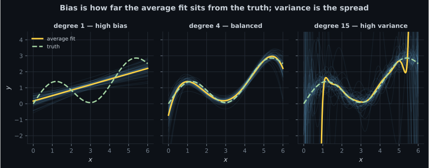
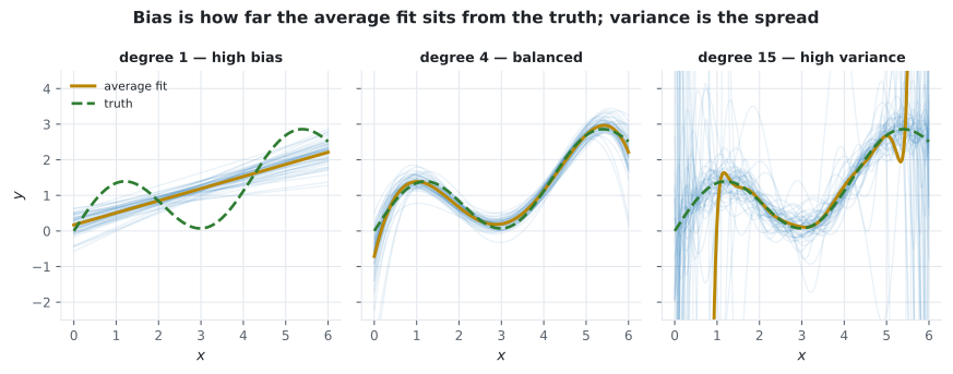
Reading the plot

• Degree 1 produces fifty almost identical lines, all of them missing the curve. Consistent and consistently wrong. More data changes nothing.
• Degree 4 tracks the truth and the spread is modest. This is what a good fit looks like when you can see the whole distribution of fits rather than one.
• Degree 15 has an average close to the truth, but individual fits swing far from it. Any single model you happen to train is a draw from that scatter.

The right panel is the crucial insight: an overfitted model is not systematically wrong, it is unreliable. Its average is fine; its individual predictions are not.

The complexity curve

figureBoth errors, against capacitymatplotlib

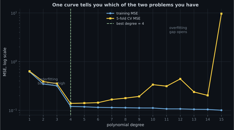
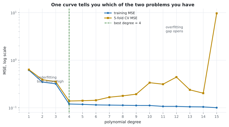
Measured on 120 points from the same generator:

Three things worth noticing:

1. Training MSE falls from 0.618 to 0.100 across the whole range and never once warns you. A model selected on training error alone would choose degree 15.
2. Degrees 4 and 6 are indistinguishable — 0.139 against 0.144. Prefer the simpler one.
3. Degree 15 is not slightly worse, it is 70 times worse. Overfitting does not degrade gracefully once the model has enough capacity to interpolate.

The learning curve

The complexity curve varies capacity at fixed data. The learning curve does the reverse, and it answers a different question: would collecting more data help?

figureFixed capacity, growing training setmatplotlib

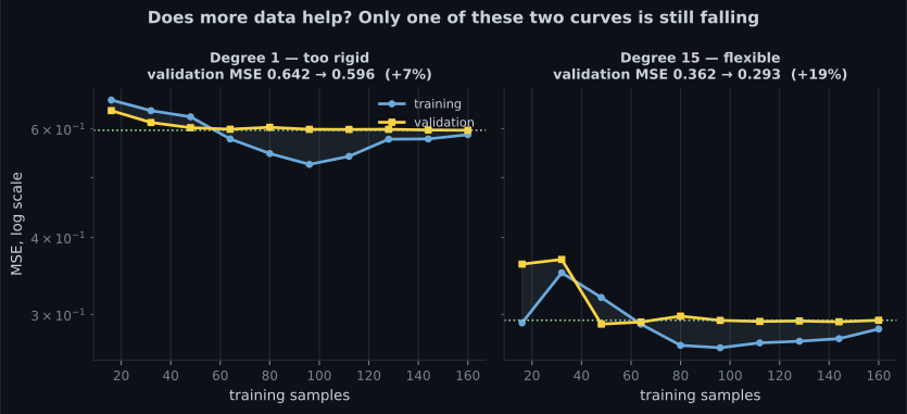
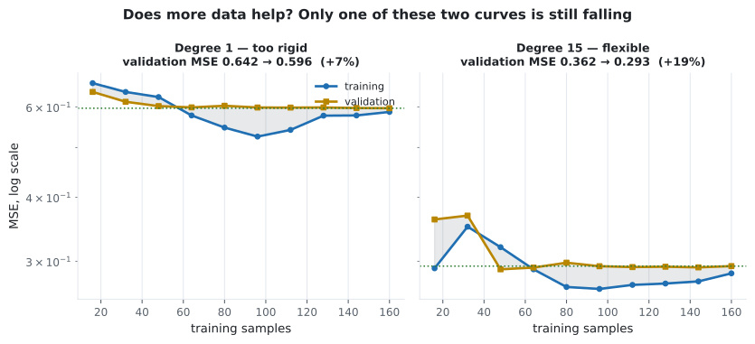
The two panels answer the same question differently:

Measured on the plot: degree 1 goes from 0.614 to 0.596 — a 3% gain from ten times the data, which is another way of saying no gain. Degree 15 goes from 0.368 to 0.294, a 20% gain and still descending. Notice also that degree 15 has stopped overfitting by 200 samples: the gap that would have been enormous at 20 samples has closed. That is data doing the work regularisation would otherwise have to do.

This is a genuinely useful business answer. “Should we spend three months labelling more data?” has a defensible answer, and it is on this plot.

Worked example by hand

Four models of the same problem, each measured on the same held-out set:

Step 1 — is the training error acceptable? Against an expert baseline of about 35,530, models A and B are already failing on the training set. That settles it: they are underfitting, and no amount of regularisation will help.

Step 2 — for the rest, how big is the gap? Model C’s training error is exactly zero, which is not an achievement but a description of what an unpruned tree does. Model D has a large gap and still the best validation score.

Step 3 — choose the fix.

• A and B: add capacity. More features, a deeper model, less regularisation.
• C: reduce capacity. max_depthmax_depth, min_samples_leafmin_samples_leaf, or pruning.
• D: more data, or mild regularisation. The gap says there is headroom; the validation score says it is still the best option available.

The trap: models A and D both need attention, and the correct actions are opposites. Applying regularisation to A — the intuitive response to “the model is not good enough” — makes it worse.

Fixing each

Underfitting

More data does not fix underfitting. A straight line fitted to a million curved points is the same straight line.

Overfitting

import numpy as np
from sklearn.linear_model import LinearRegression
from sklearn.model_selection import KFold
from sklearn.pipeline import make_pipeline
from sklearn.preprocessing import PolynomialFeatures
 
rng = np.random.default_rng(4)
x = rng.uniform(0, 6, 120)
y = np.sin(1.5 * x) + 0.35 * x + rng.normal(0, 0.35, 120)
 
folds = list(KFold(5, shuffle=True, random_state=0).split(x))
 
for degree in (1, 2, 4, 10, 15):
    train = ((y - np.polyval(np.polyfit(x, y, degree), x)) ** 2).mean()
    cv = np.mean([
        ((y[va] - np.polyval(np.polyfit(x[tr], y[tr], degree), x[va])) ** 2).mean()
        for tr, va in folds
    ])
    verdict = ("underfitting" if cv > 0.3 and cv / train < 1.5
               else "overfitting" if cv / train > 2
               else "good fit")
    print(f"degree {degree:2d}  train {train:.4f}  cv {cv:8.4f}  {verdict}")
 
# degree  1  train 0.6182  cv   0.6338  underfitting
# degree  2  train 0.3472  cv   0.3896  underfitting
# degree  4  train 0.1201  cv   0.1387  good fit
# degree 10  train 0.1117  cv   0.3368  overfitting
# degree 15  train 0.1004  cv   9.6689  overfitting

import numpy as np
from sklearn.linear_model import LinearRegression
from sklearn.model_selection import KFold
from sklearn.pipeline import make_pipeline
from sklearn.preprocessing import PolynomialFeatures
 
rng = np.random.default_rng(4)
x = rng.uniform(0, 6, 120)
y = np.sin(1.5 * x) + 0.35 * x + rng.normal(0, 0.35, 120)
 
folds = list(KFold(5, shuffle=True, random_state=0).split(x))
 
for degree in (1, 2, 4, 10, 15):
    train = ((y - np.polyval(np.polyfit(x, y, degree), x)) ** 2).mean()
    cv = np.mean([
        ((y[va] - np.polyval(np.polyfit(x[tr], y[tr], degree), x[va])) ** 2).mean()
        for tr, va in folds
    ])
    verdict = ("underfitting" if cv > 0.3 and cv / train < 1.5
               else "overfitting" if cv / train > 2
               else "good fit")
    print(f"degree {degree:2d}  train {train:.4f}  cv {cv:8.4f}  {verdict}")
 
# degree  1  train 0.6182  cv   0.6338  underfitting
# degree  2  train 0.3472  cv   0.3896  underfitting
# degree  4  train 0.1201  cv   0.1387  good fit
# degree 10  train 0.1117  cv   0.3368  overfitting
# degree 15  train 0.1004  cv   9.6689  overfitting

See it move

Pitfalls

🧪 Try It Yourself

Exercise 1 – Diagnose from two numbers

Exercise 2 – Build the complexity curve

Exercise 3 – Fix an underfitting model

Exercise 4 – Read a learning curve

Exercise 5 – Regularisation on the wrong patient

Recap

• Two numbers, never one. High-and-close is underfitting; low-with-a-gap is overfitting.
• Training error falls monotonically with capacity, so it carries no information on its own. On the measured curve it went 0.618 → 0.100 while CV error went 0.634 → 9.669.
• The complexity curve locates the best capacity; the learning curve says whether more data would help.
• An overfitted model is not systematically wrong — its average is fine and its individual predictions are unreliable.
• The fixes are opposites. Diagnose before acting: regularising an underfitting model makes it worse.
• Validation error below training error is a symptom to investigate, not a success.

Exercise 6 – Turn two numbers into a next action

Next

Continue to Bias vs Variance Tradeoff — the same two failures, derived as an exact decomposition of expected error into three terms.