
Regularization - Ridge and Lasso Regression
What you’ll learn
Section titled “What you’ll learn”- why shrinking coefficients toward zero can improve predictions — the bias-variance trade
- the Ridge closed form, and the exact shrinkage factor it applies
- the Lasso soft-thresholding rule, and why it produces genuine zeros
- both computed by hand on the orthogonal design from the Multiple Regression page
- the geometric reason a diamond selects features and a circle does not
- Elastic Net, and how to choose honestly with cross-validation
Intuition
Section titled “Intuition”Ordinary least squares has exactly one goal: make the training residuals small. Given enough features it will happily grow enormous coefficients that cancel each other out — a coefficient of +4,000 on one column and −3,950 on a nearly identical one. The training fit looks superb, and the first new row destroys it.
Regularisation adds a second goal to the objective: keep the coefficients small. The model now has to justify every unit of coefficient with a real reduction in error. Noise cannot pay that price, so noise gets squeezed out. You trade a little bias for a large reduction in variance, and on held-out data the trade usually pays.
  flowchart LR
  A["Least squares cost
fit the data"] --> C["Penalised cost"]
  B["Penalty on coefficient size
stay simple"] --> C
  C --> R["Ridge (L2): shrink everything"]
  C --> L["Lasso (L1): shrink and select"]
  C --> E["Elastic Net: both"]
The math
Section titled “The math”The three objectives
Section titled “The three objectives”Note the sums start at : the intercept is never penalised. Shrinking would tie the model’s predictions to zero rather than to the data’s mean, which is meaningless.
Ridge has a closed form
Section titled “Ridge has a closed form”Differentiating and setting the gradient to zero gives a modified Normal Equation:
Adding to the diagonal does something valuable beyond shrinkage: it makes the matrix invertible even when is singular. Ridge works when features outnumber samples, and when two columns are perfectly duplicated. Plain OLS does neither.
For an orthogonal design where , the formula collapses to pure per-coefficient shrinkage:
Every coefficient is multiplied by the same factor below 1. That factor never reaches zero for finite — which is the whole story of why Ridge cannot select features.
Lasso has no closed form, but it has a rule
Section titled “Lasso has no closed form, but it has a rule”The absolute value is not differentiable at zero, so there is no matrix formula. On an orthogonal design, though, the coordinate-wise solution is exact and beautifully simple — soft thresholding:
Subtract a fixed amount from every coefficient’s magnitude, and clamp at zero. Any coefficient smaller than the threshold becomes exactly zero, not merely small. That is feature selection falling out of the algebra.
Worked example by hand
Section titled “Worked example by hand”The orthogonal design from Multiple Linear Regression, where , and the OLS answer was .
Ridge at . With , the shrinkage factor is :
Ridge at . Factor :
Lasso at . The threshold is , subtracted from each OLS coefficient:
Lasso at . Threshold :
There it is. At Lasso has deleted the weekend feature entirely, while Ridge at the same merely shrank it to 0.357. The intercept stays at 4.25 throughout, because it is never penalised.
| OLS | Ridge | Ridge | Lasso | Lasso | |
|---|---|---|---|---|---|
| intercept | 4.25 | 4.25 | 4.25 | 4.25 | 4.25 |
| promotion | 2.25 | 1.125 | 0.643 | 1.75 | 1.00 |
| weekend | 1.25 | 0.625 | 0.357 | 0.75 | 0 |
| features used | 2 | 2 | 2 | 2 | 1 |
The geometry
Section titled “The geometry”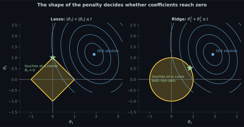
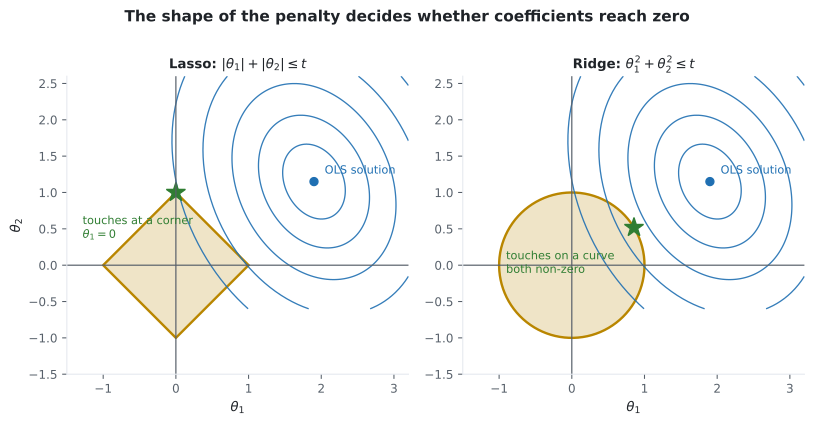
Both penalties can be restated as a constrained problem: minimise the squared error subject to the coefficient vector staying inside a region of fixed size. The solution is where the growing elliptical cost contours first touch that region.
- The ball is a diamond, and its corners sit exactly on the axes. A corner is a point where one coordinate is zero. Corners stick out, so contours tend to hit them first.
- The ball is a circle with no corners anywhere. The touch point is generically a smooth spot where every coordinate is non-zero.
That is the entire explanation, and it generalises: in dimensions the ball has low-dimensional faces where many coefficients vanish at once.
See it move
Section titled “See it move”Watch both penalties act on five coefficients as sweeps upward. The Ridge bars shrink smoothly and never disappear; the Lasso bars hit zero one after another.
From scratch
Section titled “From scratch”Both rules, verified against scikit-learn on the four-row design:
import numpy as np
from sklearn.linear_model import Ridge, Lasso

X = np.array([[-1.0, -1.0], [-1.0, 1.0], [1.0, -1.0], [1.0, 1.0]])
y = np.array([1.0, 3.0, 5.0, 8.0])
c = 4.0                                  # X.T @ X = 4 * I for this design
ols = np.array([2.25, 1.25])             # from the Multiple Regression page


def ridge_closed_form(theta_ols, lam, c):
    return c / (c + lam) * theta_ols


def lasso_soft_threshold(theta_ols, lam, c):
    shrink = lam / (2 * c)
    return np.sign(theta_ols) * np.maximum(np.abs(theta_ols) - shrink, 0.0)


for lam in (4.0, 10.0):
    mine_r = ridge_closed_form(ols, lam, c)
    mine_l = lasso_soft_threshold(ols, lam, c)

    sk_r = Ridge(alpha=lam).fit(X, y).coef_
    sk_l = Lasso(alpha=lam / (2 * len(y)), max_iter=100000).fit(X, y).coef_

    print(f"lambda = {lam}")
    print(f"  ridge  mine {mine_r.round(4)}  sklearn {sk_r.round(4)}")
    print(f"  lasso  mine {mine_l.round(4)}  sklearn {sk_l.round(4)}")

# lambda = 4.0
#   ridge  mine [1.125 0.625]  sklearn [1.125 0.625]
#   lasso  mine [1.75 0.75  ]  sklearn [1.75 0.75  ]
# lambda = 10.0
#   ridge  mine [0.6429 0.3571]  sklearn [0.6429 0.3571]
#   lasso  mine [1. 0.]         sklearn [1. 0.]
Coefficient paths on real data
Section titled “Coefficient paths on real data”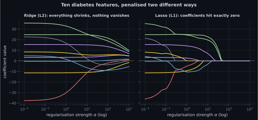
Reading the plots
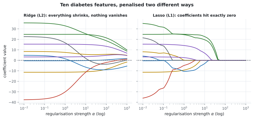
Section titled “Reading the plots”- Both start at the OLS solution. At the far left the penalty is negligible and both panels reproduce ordinary least squares.
- Ridge shrinks in proportion. The largest coefficients fall fastest in absolute terms, but the ordering is broadly preserved and nothing ever reaches the axis.
- Lasso eliminates in sequence. Each curve hits zero at its own and stays there. The order in which features drop out is a crude but genuinely useful importance ranking.
- Both end at zero. Push high enough and every coefficient vanishes; the model becomes “always predict the mean”.
With scikit-learn
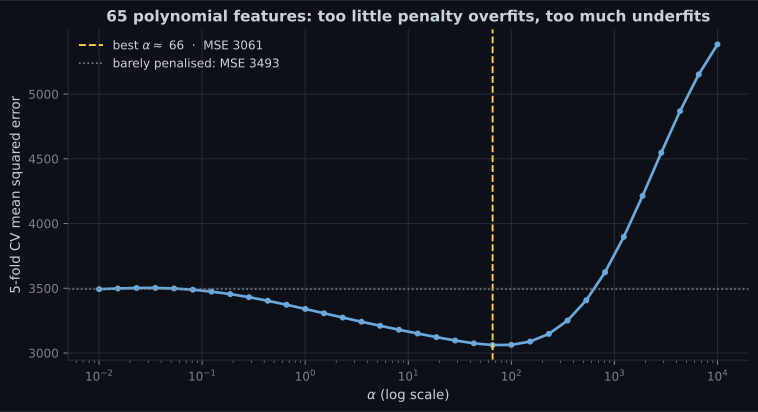
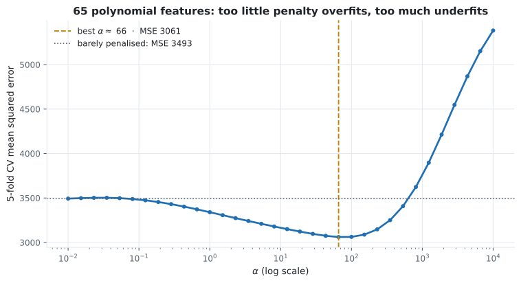
Section titled “With scikit-learn”On the raw ten diabetes features, regularisation changes almost nothing — 442 samples over 10 well-behaved columns is simply not an overfitting situation. Expand to degree 2 (65 features) and the picture changes completely:
from sklearn.datasets import load_diabetes
from sklearn.linear_model import LinearRegression, Ridge, Lasso
from sklearn.model_selection import cross_val_score
from sklearn.pipeline import make_pipeline
from sklearn.preprocessing import PolynomialFeatures, StandardScaler

X, y = load_diabetes(return_X_y=True)


def cv_mse(estimator):
    pipe = make_pipeline(
        PolynomialFeatures(2, include_bias=False),   # 10 features -> 65
        StandardScaler(),                            # penalties need a common scale
        estimator,
    )
    return -cross_val_score(
        pipe, X, y, cv=5, scoring="neg_mean_squared_error"
    ).mean()


print(f"OLS              {cv_mse(LinearRegression()):.1f}")   # OLS              3495.3
print(f"Ridge alpha=10   {cv_mse(Ridge(alpha=10)):.1f}")      # Ridge alpha=10   3165.1
print(f"Ridge alpha=100  {cv_mse(Ridge(alpha=100)):.1f}")     # Ridge alpha=100  3063.0
print(f"Lasso alpha=1    {cv_mse(Lasso(alpha=1, max_iter=200000)):.1f}")
#                                                             # Lasso alpha=1    3016.1
Regularisation cuts cross-validated error by roughly 14%, from 3495 to 3016 — and the Lasso model gets there using 34 of the 65 columns.
Choosing properly
Section titled “Choosing α\alphaα properly”import numpy as np
from sklearn.datasets import load_diabetes
from sklearn.linear_model import RidgeCV, LassoCV
from sklearn.pipeline import make_pipeline
from sklearn.preprocessing import StandardScaler
X, y = load_diabetes(return_X_y=True)
alphas = np.geomspace(1e-3, 1e3, 60)
ridge = make_pipeline(StandardScaler(), RidgeCV(alphas=alphas)).fit(X, y)
lasso = make_pipeline(
StandardScaler(), LassoCV(alphas=alphas, cv=5, max_iter=100000, random_state=0)
).fit(X, y)
print(f"RidgeCV alpha = {ridge[-1].alpha_:.4f}") # RidgeCV alpha = 1.7957
print(f"LassoCV alpha = {lasso[-1].alpha_:.4f}") # LassoCV alpha = 0.0732
print(f"Lasso kept {(lasso[-1].coef_ != 0).sum()} of 10") # Lasso kept 9 of 10RidgeCV and LassoCV do the sweep internally and are considerably faster than a manual
GridSearchCV because they reuse the solution path.
Which penalty
Section titled “Which penalty”| Ridge (L2) | Lasso (L1) | Elastic Net | |
|---|---|---|---|
| Coefficients reach zero | Never | Yes | Yes |
| Closed form | Yes | No | No |
| With correlated features | Splits weight between them | Picks one arbitrarily | Keeps the group together |
| When | Works | Selects at most features | Works, no cap |
| Interpretability | Good | Best — fewer features | Good |
| Default choice when | All features plausibly matter | You suspect most are noise | Correlated groups, or unsure |
| scikit-learn | Ridge, RidgeCV | Lasso, LassoCV | ElasticNet, ElasticNetCV |
Elastic Net exists because Lasso has a specific failure mode: with two nearly identical features it picks one at random and zeroes the other, and which one it picks flips with a different random seed. Adding a little L2 to the L1 makes correlated features enter or leave together.
pch.algoApi sklearn.linear_model.Ridge / Lasso / ElasticNet
pch.algoAssumes
- The same linearity assumptions as ordinary least squares
- Features are standardised — the penalty is meaningless otherwise
- Shrinking coefficients toward zero is a reasonable prior for this problem
pch.algoCost
- pch.algoTrain
Ridge O(m·n² + n³) closed form; Lasso O(m·n) per coordinate sweep- pch.algoPredict
O(n)- pch.algoMemory
O(n)
m = samples, n = features
pch.algoHyperparams
-
alphadefault 1.0 Penalty strength. Zero recovers OLS; large values drive every coefficient to zero. Always cross-validate it. -
l1_ratiodefault 0.5 (ElasticNet) Mix between L1 and L2. 1.0 is pure Lasso, 0.0 is pure Ridge. -
max_iterdefault 1000 Lasso and Elastic Net iterate; raise it when you see a convergence warning. -
solverdefault auto (Ridge) 'saga' handles sparse data and very large problems; 'cholesky' is fastest for dense wide-but-short data.
pch.algoReachFor
- Features outnumber samples, or nearly do
- Features are correlated and OLS coefficients look unstable
- You expanded features (polynomials, one-hot, interactions) and now overfit
- You want automatic feature selection (Lasso)
pch.algoLookElsewhere
- You have far more samples than features and OLS already generalises well
- You cannot standardise the features
- You need unbiased coefficient estimates for statistical inference
Pitfalls
Section titled “Pitfalls”-
Why can Lasso set a coefficient to exactly zero while Ridge cannot?
It is geometry. A corner of the diamond is a point where one coordinate is zero; the circle of the L2 ball has no corners, so its touch point generically has every coordinate non-zero.
pch.quizShowAnswer
B — The L1 constraint region is a diamond with corners on the axes, and the cost contours tend to touch a corner first — It is geometry. A corner of the diamond is a point where one coordinate is zero; the circle of the L2 ball has no corners, so its touch point generically has every coordinate non-zero.
-
What does adding lambda times the identity to X transpose X accomplish beyond shrinkage?
A singular X transpose X becomes non-singular once you add a positive constant to its diagonal, which is why Ridge has a solution in cases where OLS has none.
pch.quizShowAnswer
B — It makes the matrix invertible even when the features are collinear or outnumber the samples — A singular X transpose X becomes non-singular once you add a positive constant to its diagonal, which is why Ridge has a solution in cases where OLS has none.
-
Why must features be standardised before regularising?
Rescaling a feature rescales its coefficient inversely, which changes the penalty that coefficient incurs. Without a common scale you are penalising your choice of units.
pch.quizShowAnswer
B — Because the penalty charges by coefficient size, so a feature's units silently decide how much it is penalised — Rescaling a feature rescales its coefficient inversely, which changes the penalty that coefficient incurs. Without a common scale you are penalising your choice of units.
-
Your two most predictive features have a correlation of 0.98. Which penalty is the best fit?
Pure Lasso picks one of a correlated pair essentially at random. The L2 component in Elastic Net keeps the group together, which is both more stable and more interpretable.
pch.quizShowAnswer
B — Elastic Net, so the correlated pair enters or leaves together — Pure Lasso picks one of a correlated pair essentially at random. The L2 component in Elastic Net keeps the group together, which is both more stable and more interpretable.
🧪 Try It Yourself
Section titled “🧪 Try It Yourself”Exercise 1 – The Ridge shrinkage factor
Section titled “Exercise 1 – The Ridge shrinkage factor”Exercise 2 – Soft thresholding by hand
Section titled “Exercise 2 – Soft thresholding by hand”Exercise 3 – Ridge keeps everything, Lasso does not
Section titled “Exercise 3 – Ridge keeps everything, Lasso does not”Exercise 4 – Regularisation earns its keep on wide data
Section titled “Exercise 4 – Regularisation earns its keep on wide data”Exercise 5 – Let cross-validation pick alpha
Section titled “Exercise 5 – Let cross-validation pick alpha”- Regularisation adds a penalty on coefficient size, trading a little bias for a lot less variance.
- Ridge has the closed form , which also fixes singular designs.
- On an orthogonal design Ridge multiplies each coefficient by ; Lasso subtracts from each magnitude and clamps at zero.
- Worked by hand at : Ridge gives , Lasso gives — one feature deleted.
- The diamond has corners on the axes and the circle does not. That is the whole geometric story.
- On 65 polynomial features, cross-validated MSE drops from 3495 (OLS) to 3063 (Ridge) to 3016 (Lasso, using 34 columns). On the raw 10 features it changes nothing.
- Always standardise, never penalise the intercept, and always cross-validate .
Exercise 6 – Watch each penalty act on the same coefficients
Section titled “Exercise 6 – Watch each penalty act on the same coefficients”Continue to Metrics - R-Squared and Adjusted R-Squared — how to report all of this to someone who was not in the room.
pch.coffeeTagline
pch.coffeeCtapch.feedbackHeading
pch.feedbackSubheading