Eigendecomposition and Diagonalization

Diagonal matrices are the easy case for everything. Their determinant is the product of the diagonal; their $k$-th power raises each diagonal entry to the $k$; their inverse takes reciprocals. Nothing about a general matrix is that easy.

Diagonalization asks whether a given square matrix is a diagonal matrix in disguise — the same linear mapping, written in a better basis. When the answer is yes, every easy property of a diagonal matrix becomes available, and the basis that does it is the eigenbasis of §4.2.

What you’ll learn

• Definition 4.19: what diagonalizable means, and why it is exactly Chapter 2’s notion of similar.
• Why $\mathbf{A}\mathbf{P} = \mathbf{P}\mathbf{D}$ forces the columns of $\mathbf{P}$ to be eigenvectors.
• Theorem 4.20: $\mathbf{A} = \mathbf{P}\mathbf{D}\mathbf{P}^{-1}$ if and only if the eigenvectors form a basis.
• Theorem 4.21: a symmetric matrix can always be diagonalized, and by an orthogonal $\mathbf{P}$, so $\mathbf{P}^{-1} = \mathbf{P}^\top$.
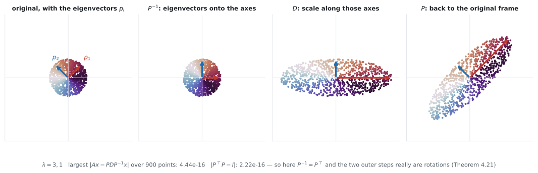
• The geometry: $\mathbf{P}^{-1}$ then $\mathbf{D}$ then $\mathbf{P}$, and what each step does to a disc.
• Equations 4.62 and 4.63: matrix powers and determinants in one line each, with a measured cost crossover.

Intuition: work in the coordinates where the map is simple

Here is the whole idea in three sentences.

A matrix does something complicated in the standard basis and something trivial in its own eigenbasis: along each eigenvector it just multiplies by a number. So if you first change coordinates into the eigenbasis, then scale each coordinate by its eigenvalue, then change back, you have applied the original matrix — by a route where the only real work is $n$ independent multiplications.

$$\mathbf{A} = \underbrace{\mathbf{P}}_{\text{change back}}\ \underbrace{\mathbf{D}}_{\text{scale}}\ \underbrace{\mathbf{P}^{-1}}_{\text{change into the eigenbasis}}$$

Read right to left, in the order a vector meets them. And the payoff arrives when you apply the matrix repeatedly: the two changes of basis cancel in the middle of $\mathbf{A}^k = \mathbf{P}\mathbf{D}\mathbf{P}^{-1}\mathbf{P}\mathbf{D}\mathbf{P}^{-1}\cdots$, leaving $\mathbf{P}\mathbf{D}^k\mathbf{P}^{-1}$.

diagram Diagram mermaid

  flowchart TD
  DIAG["a diagonal matrix D
Eq 4.49"]
  DIAG --> EASY["det = ∏dᵢᵢ · Dᵏ = each entry to the k
D⁻¹ = reciprocals, if none are zero"]
  A["a square matrix A"]
  A --> Q["is A a diagonal matrix
in a different basis?
Def 4.19: similar to a diagonal"]
  Q --> AP["AP = PD
Eq 4.50"]
  AP --> COLS["column by column: Apᵢ = λᵢpᵢ
Eq 4.53, 4.54 — so the columns
of P ARE eigenvectors"]
  COLS --> NEED["P must be invertible,
so the eigenvectors must be a BASIS"]
  NEED --> THM["Thm 4.20: A = PDP⁻¹ ⟺ the
eigenvectors form a basis of ℝⁿ"]
  THM --> SYM["Thm 4.21: symmetric ⟹ always,
and P can be ORTHOGONAL
so P⁻¹ = Pᵀ"]
  THM --> POW["Aᵏ = PDᵏP⁻¹, Eq 4.62"]
  THM --> DET["det A = ∏dᵢᵢ, Eq 4.63"]
  THM --> NO["defective ⟹ no eigendecomposition
(Jordan normal form instead —
beyond this book)"]

The math

Diagonal matrices, and why they are the target

Equation 4.49

A diagonal matrix has zeros off the diagonal:

$$\mathbf{D} = \begin{bmatrix} c_1 & \cdots & 0\\ \vdots & \ddots & \vdots\\ 0 & \cdots & c_n\end{bmatrix}$$

They allow fast computation of determinants, powers and inverses: the determinant is the product of the diagonal entries, $\mathbf{D}^k$ raises each diagonal element to the power $k$, and $\mathbf{D}^{-1}$ takes reciprocals if all of them are nonzero.

Similar, and diagonalizable

Definition 4.19 — Diagonalizable

A matrix $\mathbf{A} \in \mathbb{R}^{n\times n}$ is diagonalizable if it is similar to a diagonal matrix — that is, if there exists an invertible $\mathbf{P} \in \mathbb{R}^{n\times n}$ such that

$$\mathbf{D} = \mathbf{P}^{-1}\mathbf{A}\mathbf{P}$$

“Similar” is Chapter 2’s Definition 2.22, and §4.1 already told you what it costs: similar matrices share a determinant, a trace and — from §4.2 — a spectrum. So diagonalization does not change any of the quantities that characterise the mapping. It changes only the basis you write it in.

Why the columns of P must be eigenvectors

Take any scalars $\lambda_1, \dots, \lambda_n$ and any vectors $\mathbf{p}_1, \dots, \mathbf{p}_n$, and set $\mathbf{P} = [\mathbf{p}_1, \dots, \mathbf{p}_n]$, $\mathbf{D} = \mathrm{diag}(\lambda_1,\dots,\lambda_n)$. Multiply out both sides of $\mathbf{A}\mathbf{P} = \mathbf{P}\mathbf{D}$:

$$\mathbf{A}\mathbf{P} = \mathbf{A}[\mathbf{p}_1,\dots,\mathbf{p}_n] = [\mathbf{A}\mathbf{p}_1,\dots,\mathbf{A}\mathbf{p}_n] \tag{4.51}$$ $$\mathbf{P}\mathbf{D} = [\mathbf{p}_1,\dots,\mathbf{p}_n]\begin{bmatrix}\lambda_1 & & 0\\ & \ddots & \\ 0 & & \lambda_n\end{bmatrix} = [\lambda_1\mathbf{p}_1,\dots,\lambda_n\mathbf{p}_n] \tag{4.52}$$

Equate column by column and you get $\mathbf{A}\mathbf{p}_1 = \lambda_1\mathbf{p}_1$, …, $\mathbf{A}\mathbf{p}_n = \lambda_n\mathbf{p}_n$ (Equations 4.53 and 4.54). So

$$\mathbf{A}\mathbf{P} = \mathbf{P}\mathbf{D} \iff \lambda_1,\dots,\lambda_n \text{ are eigenvalues of } \mathbf{A} \text{ and } \mathbf{p}_1,\dots,\mathbf{p}_n \text{ the corresponding eigenvectors} \tag{4.50}$$

The eigenvectors are not chosen for the job; they are the only vectors that can do it.

The theorem, and its hypothesis

Theorem 4.20 — Eigendecomposition

A square matrix $\mathbf{A} \in \mathbb{R}^{n\times n}$ can be factored into

$$\mathbf{A} = \mathbf{P}\mathbf{D}\mathbf{P}^{-1} \tag{4.55}$$

where $\mathbf{P} \in \mathbb{R}^{n\times n}$ and $\mathbf{D}$ is a diagonal matrix whose diagonal entries are the eigenvalues of $\mathbf{A}$, if and only if the eigenvectors of $\mathbf{A}$ form a basis of $\mathbb{R}^n$.

The hypothesis is where §4.2 earns its keep. Definition 4.19 needs $\mathbf{P}$ invertible, so $\mathbf{P}$ needs full rank (§4.1, Theorem 4.3), so its $n$ columns need to be linearly independent — so there must be $n$ linearly independent eigenvectors. That is exactly the negation of defective (Definition 4.13).

So: only non-defective matrices can be diagonalized, and the columns of $\mathbf{P}$ are the $n$ eigenvectors. A repeated eigenvalue is fine as long as its eigenspace is big enough; a repeated eigenvalue whose geometric multiplicity falls short is fatal.

Theorem 4.21

A symmetric matrix $\mathbf{S} \in \mathbb{R}^{n\times n}$ can always be diagonalized.

This follows directly from the spectral theorem (4.15), and it comes with a bonus: the spectral theorem gives an orthonormal basis of eigenvectors, so $\mathbf{P}$ can be taken orthogonal, and then

$$\mathbf{D} = \mathbf{P}^\top\mathbf{A}\mathbf{P}$$

with no inverse to compute. That substitution — $\mathbf{P}^{-1} \to \mathbf{P}^\top$ — is why every covariance and kernel matrix in the applied chapters is handled without an inverse anywhere in sight.

The Jordan normal form is out of scope

The book’s Remark: for defective matrices there is a decomposition that does work, the Jordan normal form, and it is beyond the scope of the book. It is worth knowing the name so you recognise that “cannot be diagonalized” is not the end of the story mathematically — only the end of what this book needs.

The geometry

The book’s Figure 4.7 reads as a loop, and it is worth walking round it.

step	what it does
$\mathbf{P}^{-1}$	a change of basis from the standard basis into the eigenbasis: it maps the eigenvectors $\mathbf{p}_i$ onto the standard basis vectors $\mathbf{e}_i$
$\mathbf{D}$	scales along those axes by the eigenvalues $\lambda_i$ — a circle becomes an axis-aligned ellipse
$\mathbf{P}$	undoes the basis change, returning the scaled vectors to the original frame, giving $\lambda_i\mathbf{p}_i$

For a symmetric matrix the two outer steps are genuine rotations (or reflections), because $\mathbf{P}$ is orthogonal. For a general non-defective matrix they are not — $\mathbf{P}$ is invertible but need not be orthogonal, so the “change of basis” also shears. The book draws the symmetric case, which is why its Figure 4.7 looks like rotate-scale-rotate.

What it buys

Equations 4.62 and 4.63

Powers.

$$\mathbf{A}^k = (\mathbf{P}\mathbf{D}\mathbf{P}^{-1})^k = \mathbf{P}\mathbf{D}^k\mathbf{P}^{-1}$$

because the inner $\mathbf{P}^{-1}\mathbf{P}$ pairs cancel. Computing $\mathbf{D}^k$ is $n$ scalar powers.

Determinants.

$$\det(\mathbf{A}) = \det(\mathbf{P}\mathbf{D}\mathbf{P}^{-1}) = \det(\mathbf{P})\det(\mathbf{D})\det(\mathbf{P}^{-1}) = \det(\mathbf{D}) = \prod_i d_{ii}$$

using $\det(\mathbf{P}^{-1}) = 1/\det(\mathbf{P})$ from §4.1.

The determinant identity is Theorem 4.16 again, arriving by a different route. The power identity is new, and it is the practical reason to diagonalize.

From the book

Section 4.4. Equation 4.49 defines a diagonal matrix and lists what it makes easy. Definition 4.19 gives diagonalizability by reference to Chapter 2’s Definition 2.22 (similar matrices). Equations 4.50 to 4.54 derive $\mathbf{A}\mathbf{P} = \mathbf{P}\mathbf{D}$ column by column, showing the columns of $\mathbf{P}$ must be eigenvectors, and note that invertibility of $\mathbf{P}$ requires $n$ linearly independent ones. Theorem 4.20 (Equation 4.55) is the eigendecomposition, with the observation that only non-defective matrices can be diagonalized. Theorem 4.21 handles symmetric matrices, with the note that the spectral theorem makes $\mathbf{P}$ orthogonal so that $\mathbf{D} = \mathbf{P}^\top\mathbf{A}\mathbf{P}$, and a Remark points to the Jordan normal form for the defective case. Figure 4.7 gives the geometric intuition as $\mathbf{P}^{-1}$, then $\mathbf{D}$, then $\mathbf{P}$. Example 4.11 (Equations 4.56 to 4.61) works a $2\times2$ in three steps. Equations 4.62 and 4.63 give matrix powers and the determinant.

Worked example by hand

Example 4.11

$$\mathbf{A} = \begin{bmatrix}2 & 1\\ 1 & 2\end{bmatrix}$$

Step 1 — eigenvalues and eigenvectors.

$$\det(\mathbf{A}-\lambda\mathbf{I}) = \begin{vmatrix}2-\lambda & 1\\ 1 & 2-\lambda\end{vmatrix} = (2-\lambda)^2 - 1 = \lambda^2 - 4\lambda + 3 = (\lambda-3)(\lambda-1) \tag{4.56b}$$

so $\lambda_1 = 1$ and $\lambda_2 = 3$. Solving $\begin{bmatrix}2&1\\1&2\end{bmatrix}\mathbf{p}_i = \lambda_i\mathbf{p}_i$ and normalising:

$$\mathbf{p}_1 = \frac{1}{\sqrt2}\begin{bmatrix}1\\-1\end{bmatrix}, \qquad \mathbf{p}_2 = \frac{1}{\sqrt2}\begin{bmatrix}1\\1\end{bmatrix} \tag{4.58}$$

Step 2 — check existence. Two distinct eigenvalues, so by Theorem 4.12 the eigenvectors are independent, so they form a basis of $\mathbb{R}^2$, so Theorem 4.20 applies.

Step 3 — assemble.

$$\mathbf{P} = [\mathbf{p}_1, \mathbf{p}_2] = \frac{1}{\sqrt2}\begin{bmatrix}1 & 1\\ -1 & 1\end{bmatrix} \tag{4.59}$$ $$\mathbf{P}^{-1}\mathbf{A}\mathbf{P} = \begin{bmatrix}1 & 0\\ 0 & 3\end{bmatrix} = \mathbf{D} \tag{4.60}$$

And because $\mathbf{A}$ is symmetric, the eigenvectors are already an ONB, so $\mathbf{P}^{-1} = \mathbf{P}^\top$ and the factorisation can be written without an inverse (Equation 4.61):

$$\underbrace{\begin{bmatrix}2&1\\1&2\end{bmatrix}}_{\mathbf{A}} = \underbrace{\frac{1}{\sqrt2}\begin{bmatrix}1&1\\-1&1\end{bmatrix}}_{\mathbf{P}} \underbrace{\begin{bmatrix}1&0\\0&3\end{bmatrix}}_{\mathbf{D}} \underbrace{\frac{1}{\sqrt2}\begin{bmatrix}1&-1\\1&1\end{bmatrix}}_{\mathbf{P}^\top}$$

Verified numerically: $\mathbf{P}^{-1} = \mathbf{P}^\top$ exactly, and $\mathbf{P}\mathbf{D}\mathbf{P}^\top$ reproduces $\mathbf{A}$ to $4.44\times10^{-16}$.

A closed form for the k-th power

Equation 4.62 does something a matrix multiply cannot: it gives an algebraic formula. For this $\mathbf{A}$,

$$\mathbf{A}^k = \mathbf{P}\begin{bmatrix}1^k & 0\\ 0 & 3^k\end{bmatrix}\mathbf{P}^\top = \frac{1}{2}\begin{bmatrix}1 + 3^k & -1 + 3^k\\ -1 + 3^k & 1 + 3^k\end{bmatrix}$$

Read off the top-left entry: $(\mathbf{A}^k)_{11} = \tfrac{1}{2}(1 + 3^k)$. Check against direct multiplication:

$k$	direct $\mathbf{A}^k$, entry $(1,1)$	$\tfrac12(1+3^k)$
1	$2$	$2$
2	$5$	$5$
5	$122$	$122$
10	$29525$	$29525$
20	$1743392201$	$1743392201$

Every value integer and exact. That is what a diagonalisation gives you that repeated multiplication does not: not a faster loop, a formula.

example_411.py

import numpy as np
 
A = np.array([[2.0, 1.0], [1.0, 2.0]])
 
# The book's P and D (Equations 4.58 to 4.60).
P = np.array([[1.0, 1.0], [-1.0, 1.0]]) / np.sqrt(2)
D = np.diag([1.0, 3.0])
 
print("P^-1 A P ="); print(np.round(np.linalg.inv(P) @ A @ P, 10))
print("P^-1 equals P^T:", np.allclose(np.linalg.inv(P), P.T))
print("P D P^T - A, largest entry:", f"{float(np.abs(P @ D @ P.T - A).max()):.2e}")
 
print()
print("Equation 4.62, against direct multiplication:")
for k in (1, 2, 5, 10, 20):
    direct = np.linalg.matrix_power(A, k)
    via = P @ np.diag([1.0 ** k, 3.0 ** k]) @ P.T
    closed = (1 + 3.0 ** k) / 2
    print(f"  k={k:3}  direct[0,0] {direct[0, 0]:16.1f}  PD^kP^T {via[0, 0]:16.1f}  "
          f"(1+3^k)/2 {closed:16.1f}  gap {float(np.abs(direct - via).max()):.2e}")
 
print()
print("Equation 4.63: det A =", float(np.linalg.det(A)), " product of D's diagonal =", float(np.prod(np.diag(D))))

output

P^-1 A P =
[[ 1.  0.]
 [-0.  3.]]
P^-1 equals P^T: True
P D P^T - A, largest entry: 4.44e-16
 
Equation 4.62, against direct multiplication:
  k=  1  direct[0,0]              2.0  PD^kP^T              2.0  (1+3^k)/2              2.0  gap 4.44e-16
  k=  2  direct[0,0]              5.0  PD^kP^T              5.0  (1+3^k)/2              5.0  gap 8.88e-16
  k=  5  direct[0,0]            122.0  PD^kP^T            122.0  (1+3^k)/2            122.0  gap 1.42e-14
  k= 10  direct[0,0]          29525.0  PD^kP^T          29525.0  (1+3^k)/2          29525.0  gap 3.64e-12
  k= 20  direct[0,0]     1743392201.0  PD^kP^T     1743392201.0  (1+3^k)/2     1743392201.0  gap 2.38e-07
 
Equation 4.63: det A = 2.9999999999999996  product of D's diagonal = 3.0

Two things worth noticing. The absolute gap grows to $2.4\times10^{-7}$ by $k = 20$ — but $\mathbf{A}^{20}$ has entries around $1.7\times10^{9}$, so that is a relative error of about $10^{-16}$, which is machine precision, not degradation. And the last line: $\det\mathbf{A}$ from an LU factorisation gives $2.9999999999999996$ where the product of the eigenvalues gives exactly $3$.

See it move

The first sketch is the three-step loop with a slider that interpolates through it, so you can see which step does what.

sketch P-inverse, then D, then P p5.js Pause Restart

Drag the stage slider to move a disc of points through the three factors. The eigenvectors are marked: P-inverse lands them on the coordinate axes, D stretches along those axes, and P returns everything to the original frame. Edit the matrix — keep it symmetric with the off-diagonal knob, or break symmetry and watch the outer steps stop being rotations.

The second sketch is the payoff: watch $\mathbf{A}^k$ collapse onto the dominant eigendirection.

sketch A to the k collapses onto the dominant eigenvector p5.js Pause Restart

Drag k. The disc is repeatedly transformed by A, computed as P D-to-the-k P-inverse. Because one eigenvalue dominates, everything is squeezed towards a single line — and the readout shows the ratio of the two eigenvalues raised to the k, which is exactly how fast that happens.

And the stepped version on Example 4.11, with the det/trace checks and the diagonalisability verdict:

matrixExample 4.11, step by stepeigen analysis, §4.2

A

2112

1p(L) = det(A - L*I)                 # the characteristic polynomial, Def 4.52roots = solve(p)                    # the eigenvalues, Thm 4.83for L in roots:4    E_L = null_space(A - L*I)       # the eigenspace, Def 4.105    check A @ v == L * v for v in E_L6det(A) == prod(roots)               # Thm 4.167trace(A) == sum(roots)              # Thm 4.178diagonalizable iff sum(dim E_L) == n   # Thm 4.20

setupA is 2x2. The eigenvalue equation Ax = Lx asks for directions the matrix only scales — and the only way a nonzero x can satisfy (A - L I)x = 0 is for A - L I to be singular, so det(A - L I) = 0 is where the eigenvalues must come from.

Play‹›1/7⟲

Symmetric, two distinct eigenvalues, orthogonal eigenvectors — the case Theorem 4.21 guarantees. The final frame confirms the eigenspace dimensions add to 2.

From scratch

eigendecomposition_from_scratch.py

import numpy as np
 
def eigendecompose(A, tol=1e-8):
    """Theorem 4.20, with its hypothesis actually checked."""
    A = np.asarray(A, dtype=float)
    n = A.shape[0]
    symmetric = bool(np.allclose(A, A.T))
 
    # Theorem 4.21: for symmetric input use eigh, which returns an ONB.
    vals, vecs = (np.linalg.eigh(A) if symmetric else np.linalg.eig(A))
 
    if np.any(np.abs(np.imag(vals)) > 1e-12):
        raise ValueError("complex eigenvalues: not diagonalizable over the reals")
 
    vals = np.real(vals)
    vecs = np.real(vecs)
 
    # The hypothesis: do the eigenvectors form a basis?
    independent = 0
    for lam in np.unique(np.round(vals, 8)):
        independent += n - np.linalg.matrix_rank(A - lam * np.eye(n), tol=tol)
    if independent < n:
        raise ValueError(f"defective: {independent} independent eigenvectors, {n} needed")
 
    P, D = vecs, np.diag(vals)
    Pinv = P.T if symmetric else np.linalg.inv(P)
    return P, D, Pinv, symmetric
 
cases = {
    "Ex 4.11 [[2,1],[1,2]]":  [[2.0, 1], [1, 2]],
    "Ex 4.5  [[4,2],[1,3]]":  [[4.0, 2], [1, 3]],
    "Ex 4.6  [[2,1],[0,2]]":  [[2.0, 1], [0, 2]],
    "Ex 4.8  3x3 symmetric":  [[3.0, 2, 2], [2, 3, 2], [2, 2, 3]],
    "rotation by 30 deg":     [[np.cos(np.pi / 6), -np.sin(np.pi / 6)],
                               [np.sin(np.pi / 6), np.cos(np.pi / 6)]],
}
 
for name, A in cases.items():
    A = np.asarray(A, dtype=float)
    try:
        P, D, Pinv, sym = eigendecompose(A)
        gap = float(np.abs(P @ D @ Pinv - A).max())
        orth = float(np.abs(P.T @ P - np.eye(A.shape[0])).max())
        print(f"{name:24} OK   symmetric {str(sym):5} "
              f"|P D P^-1 - A| {gap:.1e}  |P^T P - I| {orth:.1e}  "
              f"det from D {float(np.prod(np.diag(D))):+.4f}")
    except ValueError as e:
        print(f"{name:24} NO   {e}")

output

Ex 4.11 [[2,1],[1,2]]    OK   symmetric True  |P D P^-1 - A| 4.4e-16  |P^T P - I| 2.2e-16  det from D +3.0000
Ex 4.5  [[4,2],[1,3]]    OK   symmetric False |P D P^-1 - A| 8.9e-16  |P^T P - I| 3.2e-01  det from D +10.0000
Ex 4.6  [[2,1],[0,2]]    NO   defective: 1 independent eigenvectors, 2 needed
Ex 4.8  3x3 symmetric    OK   symmetric True  |P D P^-1 - A| 3.6e-15  |P^T P - I| 5.6e-16  det from D +7.0000
rotation by 30 deg       NO   complex eigenvalues: not diagonalizable over the reals

The column to read is $\lVert\mathbf{P}^\top\mathbf{P} - \mathbf{I}\rVert$. For the two symmetric matrices it is at machine precision — $\mathbf{P}$ is orthogonal, exactly as Theorem 4.21 promises. For the non-symmetric Example 4.5 it is $0.3162$: $\mathbf{P}$ is perfectly invertible and the decomposition is perfectly valid, but the change of basis is not a rotation — the two eigendirections meet at $71.6°$ rather than $90°$, so their inner product is $-0.3162$ instead of $0$. That is the difference between Theorem 4.20 and Theorem 4.21, visible as one number.

On real data

figure The book's Figure 4.7, rebuilt matplotlib

Eigenvalues 3 and 1. Measured over 900 points, the largest gap between the direct product A x and the three-step chain is 4.44e-16, and P-transpose P differs from the identity by 2.22e-16 — so here the two outer steps really are rotations.

figure Equation 4.62, measured matplotlib

Over powers up to 1000 the two routes never disagree by more than 9.66e-15 relative. On the right, for n = 6 the eigen route becomes cheaper at k = 14 — one decomposition plus k scalar powers against k matrix products.

figure Theorem 4.20's hypothesis, quantified matplotlib

Four thousand 4x4 matrices attempted per construction. Random Gaussian entries are never defective; small integer entries are 2.675% of the time, because exact repeats become possible; a deliberately repeated eigenvalue is still never defective; only a Jordan block is, at 99.37%.

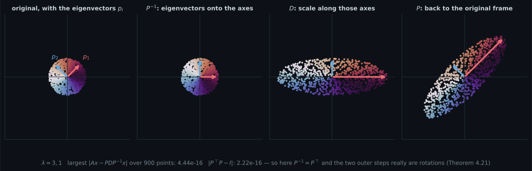
Reading the plot

From the three-step figure. The eigenvector arrows are the thing to follow. In the first panel they point in two oblique directions; in the second they lie on the coordinate axes, which is what “change into the eigenbasis” means; in the third they have been stretched by $3$ and $1$; in the fourth they are back where they started, longer. The disc becomes an ellipse whose axes are the eigenvectors — and it becomes axis-aligned only in the middle two panels.

The measured numbers close the loop: the largest disagreement between $\mathbf{A}\mathbf{x}$ and the three-step chain, over $900$ points, is $4.44\times10^{-16}$. And $\lVert\mathbf{P}^\top\mathbf{P} - \mathbf{I}\rVert = 2.22\times10^{-16}$, confirming the matrix is symmetric enough for $\mathbf{P}^{-1} = \mathbf{P}^\top$ to be used.

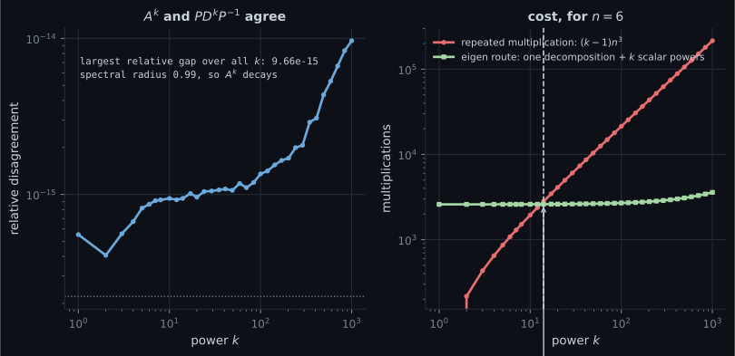
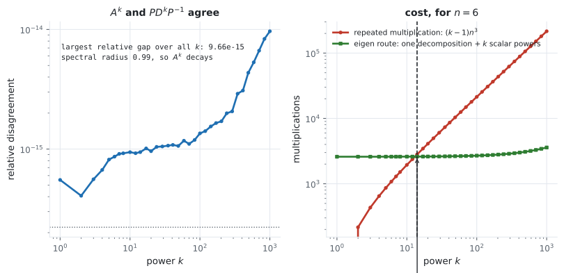
From the matrix-power figure. Two separate claims.

Accuracy. Over a thousand powers the two routes agree to $9.66\times10^{-15}$ relative. There is no drift: repeated multiplication accumulates rounding error and the eigen route accumulates a different rounding error, and both stay at machine precision because this matrix has spectral radius $0.99$ and its powers decay rather than grow.

Cost. The crossover for $n = 6$ is $k = 14$, and it is worth reading the counts rather than the curves: at $k = 13$ repeated multiplication needs $2592$ multiplications against the eigen route’s $2605$; at $k = 14$ it is $2808$ against $2606$. The eigen route pays a large fixed cost — about $12n^3$ for the decomposition plus reassembly — and then almost nothing per power.

But the real argument for Equation 4.62 is not the flop count. It is that the eigen route gives an algebraic answer: $(\mathbf{A}^k)_{11} = \tfrac12(1+3^k)$ for the worked example, valid for every $k$ at once, which no amount of matrix multiplication produces.

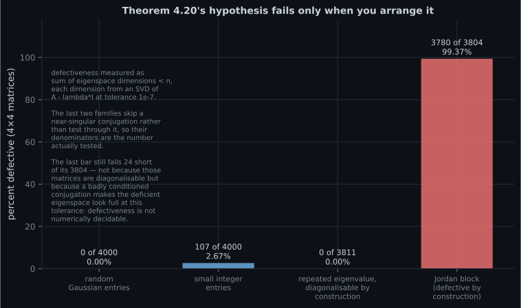
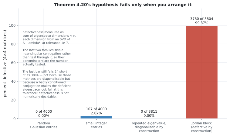
From the defectiveness figure. This is the figure that recalibrates the hypothesis. Textbooks introduce “non-defective” as a condition to worry about, and the measurement says:

construction	percent defective
random Gaussian entries	$0.000\%$ ($0$ of $4000$)
small integer entries	$2.675\%$ ($107$ of $4000$)
built with a repeated eigenvalue, diagonalizable by construction	$0.000\%$ ($0$ of $3811$)
a Jordan block, defective by construction	$99.37\%$ ($3780$ of $3804$)

The last two denominators are smaller because those two families conjugate a diagonal matrix by a random $\mathbf{S}$ and skip the draw when $\lvert\det\mathbf{S} vert < 0.1$ rather than test through a near-singular conjugation. Counting a skipped draw as non-defective would have shown the last bar at $94.5\%$ and made a missing sample look like a numerical effect.

Defectiveness is not something random matrices do. It requires an exactly repeated eigenvalue, which requires exact arithmetic coincidences — so it happens for small-integer matrices $2.7\%$ of the time and essentially never for continuous entries. What it is common in is structured matrices, which is where your data actually comes from.

Even so the last bar falls $24$ short of its $3804$. That residue is not a counterexample — it is the tolerance. A badly conditioned conjugation makes the deficient eigenspace look full at any fixed threshold, which is the pitfall below.

Pitfalls

Defectiveness is not numerically decidable

The measurement above is the proof: matrices constructed to be defective are reported non-defective $24$ times in $3804$, and every one of those $24$ genuinely is defective. Geometric multiplicity is the nullity of $\mathbf{A}-\lambda\mathbf{I}$, nullity needs a rank tolerance, and near-defective is indistinguishable from defective at any tolerance you pick. In practice you do not test for defectiveness — you use the SVD, which needs no such hypothesis.

np.linalg.eig does not tell you whether the decomposition is valid

It returns $\mathbf{P}$ and $\mathbf{D}$ for a defective matrix too, with a $\mathbf{P}$ that is singular or nearly so. np.linalg.eig(np.array([[2.,1],[0,2]])) returns two columns that are the same vector up to sign — a rank-1 $\mathbf{P}$ with condition number $4.5\times10^{15}$ — and $\mathbf{P}\mathbf{D}\mathbf{P}^{-1}$ then reconstructs a matrix that is off by $1.0$, the size of the off-diagonal entry it silently dropped. Nothing raises. Check the condition number of $\mathbf{P}$ before trusting a reconstruction.

Use eigh for symmetric input, and never on non-symmetric input

For a symmetric matrix eigh is faster, returns real values in ascending order, and returns an orthonormal $\mathbf{P}$ so you can write $\mathbf{P}^\top$ instead of inverting. Handed a non-symmetric matrix it reads only the lower triangle and returns confident nonsense. eig is the general tool and returns complex arrays even when every eigenvalue is real.

An orthogonal P is a property of symmetry, not of diagonalizability

Example 4.5 is diagonalizable with $\lVert\mathbf{P}^\top\mathbf{P}-\mathbf{I}\rVert = 0.3162$. Theorem 4.20 gives you an invertible $\mathbf{P}$; only Theorem 4.21, via the spectral theorem, gives an orthogonal one. Code that assumes $\mathbf{P}^{-1} = \mathbf{P}^\top$ without checking symmetry is wrong by $0.32$ here.

Repeated eigenvalues make P non-unique in a way that breaks reproducibility

Any orthogonal rotation within a repeated eigenspace gives an equally valid $\mathbf{P}$. Example 4.8’s $\lambda = 1$ eigenspace is two-dimensional, so its two columns of $\mathbf{P}$ are determined only up to a rotation in that plane — and different LAPACK builds may pick different ones. Anything downstream that reads individual eigenvector components (a PCA loading plot, a saved projection) is unstable under a repeated or nearly-repeated eigenvalue.

Do not diagonalize just to compute a determinant

Equation 4.63 is a lovely identity and a poor algorithm: an eigendecomposition costs about $10n^3$ where an LU factorisation costs $2n^3/3$, and it is less accurate — measured here, $2.9999999999999996$ from LU against exactly $3$ from the eigenvalues on a $2\times2$, but the ordering reverses on larger ill-conditioned input. Use Cholesky if the matrix is SPD, LU otherwise.

Compare

	eigendecomposition $\mathbf{P}\mathbf{D}\mathbf{P}^{-1}$	SVD $\mathbf{U}\boldsymbol{\Sigma}\mathbf{V}^\top$
exists for	square and non-defective	every matrix
shape	one space to itself	domain to codomain, possibly different dimensions
outer factors	invertible, generally not orthogonal	both orthogonal, so both are rotations
are the outer factors inverse to each other?	yes, $\mathbf{P}$ and $\mathbf{P}^{-1}$	no — different spaces
middle factor	eigenvalues, possibly negative or complex	singular values, real and non-negative
for a symmetric positive definite matrix	the same thing	the same thing
gives matrix powers?	yes, $\mathbf{P}\mathbf{D}^k\mathbf{P}^{-1}$	not directly
gives best low-rank approximation?	no	yes, §4.6

The last two rows are why both exist. §4.5 takes up the right-hand column.

pch.quizTag Check your understanding

1. Why must the columns of P be eigenvectors, rather than merely some convenient basis?

   A Convention B Because multiplying out AP = PD column by column gives A p-i = lambda-i p-i for every i — the equation itself forces it, and nothing else satisfies it C Because eigenvectors are orthogonal D Because D must be diagonal
   pch.quizShowAnswer

   B — Because multiplying out AP = PD column by column gives A p-i = lambda-i p-i for every i — the equation itself forces it, and nothing else satisfies it — Equations 4.51 and 4.52 do the multiplication. AP has columns A p-i and PD has columns lambda-i p-i, so equating them is the eigenvalue equation n times over.

2. Theorem 4.20's hypothesis is that the eigenvectors form a basis. Where does that requirement come from?

   A From the spectral theorem B From needing P to be invertible: Definition 4.19 requires an invertible P, invertible means full rank, and full rank for an n by n matrix means n linearly independent columns — which are the eigenvectors C From needing D to be diagonal D From needing the eigenvalues to be real
   pch.quizShowAnswer

   B — From needing P to be invertible: Definition 4.19 requires an invertible P, invertible means full rank, and full rank for an n by n matrix means n linearly independent columns — which are the eigenvectors — So the hypothesis is exactly the negation of Definition 4.13's 'defective'. Distinct eigenvalues are sufficient by Theorem 4.12 but not necessary; what matters is that the eigenspace dimensions add to n.

3. For Example 4.5, [[4,2],[1,3]], the decomposition works but P-transpose P differs from the identity by 0.3162. What does that mean?

   A The decomposition is invalid B P is invertible, so Theorem 4.20 holds, but the matrix is not symmetric so Theorem 4.21 does not apply and P is not orthogonal — meaning P-inverse is not P-transpose and the change of basis shears as well as turns C The eigenvalues are wrong D The matrix is defective
   pch.quizShowAnswer

   B — P is invertible, so Theorem 4.20 holds, but the matrix is not symmetric so Theorem 4.21 does not apply and P is not orthogonal — meaning P-inverse is not P-transpose and the change of basis shears as well as turns — The reconstruction gap is 8.9e-16, so the factorisation is fine. Only the symmetric cases in that table have P-transpose P at machine precision, which is Theorem 4.21 being the stronger statement.

4. Random 4x4 Gaussian matrices were never defective in 4000 trials; small-integer ones were 2.7% of the time. Why the difference?

   A Integers are harder to diagonalise B Defectiveness needs an exactly repeated eigenvalue, which needs an exact arithmetic coincidence — impossible for continuous entries and merely uncommon for a small integer range C The tolerance was different D Gaussian matrices are symmetric
   pch.quizShowAnswer

   B — Defectiveness needs an exactly repeated eigenvalue, which needs an exact arithmetic coincidence — impossible for continuous entries and merely uncommon for a small integer range — Which recalibrates the hypothesis: defectiveness is not a hazard of random data, it is a hazard of structured data, and structured is where real matrices come from.

5. The eigen route to A-to-the-k becomes cheaper than repeated multiplication at k = 14 for n = 6. Is that the main argument for Equation 4.62?

   A Yes, the flop count is the point B No. The stronger argument is that it gives an algebraic formula — for the worked example the (1,1) entry of A-to-the-k is exactly one half of one plus three to the k, valid for every k at once, which no number of matrix multiplications produces C No, the point is accuracy D No, the point is that it needs less memory
   pch.quizShowAnswer

   B — No. The stronger argument is that it gives an algebraic formula — for the worked example the (1,1) entry of A-to-the-k is exactly one half of one plus three to the k, valid for every k at once, which no number of matrix multiplications produces — The measured values confirm the formula: 2, 5, 122, 29525 and 1743392201 at k = 1, 2, 5, 10 and 20. The flop crossover is real but secondary.

🧪 Try It Yourself

Exercise 1 – Example 4.11 in three steps

pch.exerciseTag pch.exerciseTitle

Exercise 2 – A closed form for the k-th power

pch.exerciseTag pch.exerciseTitle

Exercise 3 – Check the hypothesis before trusting the factorisation

pch.exerciseTag pch.exerciseTitle

Exercise 4 – What numpy does with a defective matrix

pch.exerciseTag pch.exerciseTitle

Exercise 5 – Powers collapse onto the dominant eigenvector

pch.exerciseTag pch.exerciseTitle

Recall card

• Diagonalizable means similar to a diagonal matrix: there is an invertible P with D equal to P-inverse A P, and similar matrices share their determinant, trace and spectrum.
• The columns of P must be eigenvectors, because multiplying out A P = P D column by column gives the eigenvalue equation n times over.
• Theorem 4.20 is an if and only if: the factorisation exists exactly when the eigenvectors form a basis — that is, exactly when the matrix is not defective.
• Theorem 4.21: a symmetric matrix can always be diagonalized, and the spectral theorem makes P orthogonal, so P-inverse becomes P-transpose and no inverse is ever computed.
• The geometry is three steps: P-inverse changes into the eigenbasis, D scales along those axes, P changes back. Only for a symmetric matrix are the two outer steps rotations.
• A to the k equals P D-to-the-k P-inverse, because the inner pairs cancel — and that gives an algebraic formula, not merely a faster loop.
• The determinant is the product of D’s diagonal, which is Theorem 4.16 arriving by another route.
• Defectiveness is rare in random matrices and common in structured ones: zero of four thousand Gaussian matrices, 2.675 percent of small-integer ones, and 99.37 percent of Jordan blocks — and it is not numerically decidable, since a badly conditioned conjugation makes a deficient eigenspace look full at any fixed tolerance.
• P orthogonal follows from symmetry, not from diagonalizability. For the non-symmetric Example 4.5, P-transpose P differs from the identity by 0.3162, because its two eigendirections meet at 71.6 degrees rather than 90.
• Repeated eigenvalues make P non-unique up to a rotation within the eigenspace, which is a reproducibility hazard for anything reading individual eigenvector components.

Next: Singular Value Decomposition — the same idea with both hypotheses dropped.