PCA in High Dimensions

§10.4 asked how to compute the eigenvectors. §10.5 asks a sharper question: is $\mathbf{S}$ even the right matrix to decompose?

For example, if our $\mathbf{x}_n$ are images with $10{,}000$ pixels (e.g., $100 \times 100$ pixel images), we would need to compute the eigendecomposition of a $10{,}000 \times 10{,}000$ covariance matrix.

That matrix is $0.75$ GiB and its decomposition is cubic in $D$. If you have $50$ images, almost all of it is zeros.

What you’ll learn

• Why $N \ll D$ makes $\mathbf{S}$ enormously redundant — and exactly how redundant: measured, a $784\times784$ covariance built from $50$ points has $735$ eigenvalues at machine zero.
• Equation 10.56’s substitution $\mathbf{c}_m := \mathbf{X}^\top\mathbf{b}_m$, turning a $D\times D$ eigenproblem into an $N\times N$ one with the same nonzero eigenvalues — measured agreement $3.4\times10^{-13}$.
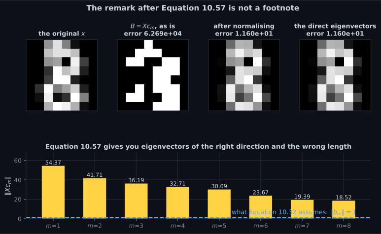
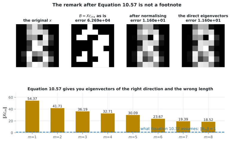
• Equation 10.57’s recovery of $\mathbf{b}_m$ from $\mathbf{c}_m$, and the one-line remark after it that is not optional: measured, skipping the normalisation turns a reconstruction error of $1.160\times10^{1}$ into $6.269\times10^{4}$.
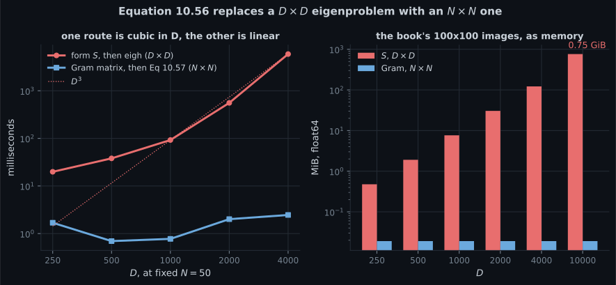
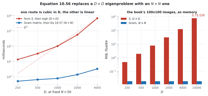
• What it actually saves: $47.9\times$ at $D = 500$ rising to $\mathbf{4565\times}$ at $D = 4000$, with the top five eigenvalues agreeing to $5.5\times10^{-12}$; and $0.75$ GiB of memory against $19.5$ KiB.
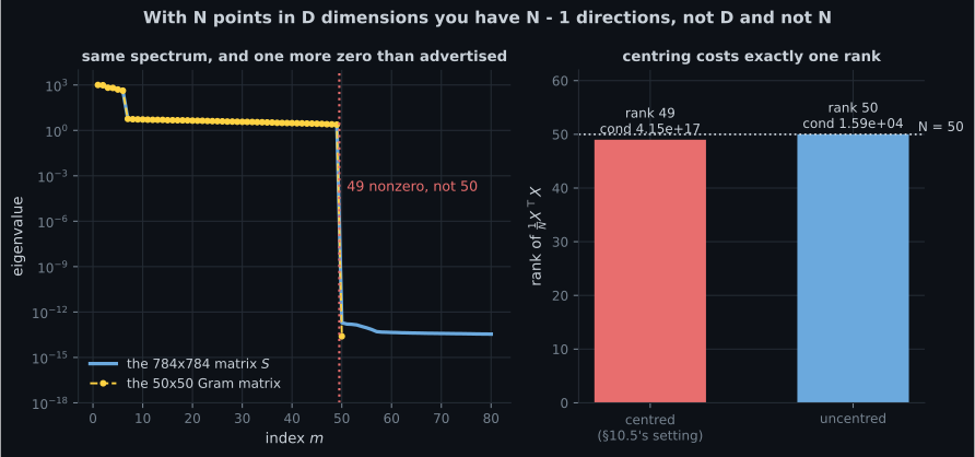
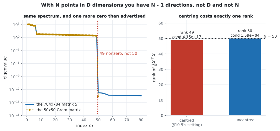
• Two claims in §10.5 that centred data contradicts. The book says the rank of $\mathbf{S}$ is $N$, and that $\frac{1}{N}\mathbf{X}^\top\mathbf{X}$ “has rank $N$ and is invertible”. Both are off by one: centring puts $\mathbf{1}$ in the null space, so the rank is $N-1$ and the Gram matrix is singular — measured condition number $4.15\times10^{17}$.
• Why §10.8 says this idea “can be pushed to the extreme”: the $N\times N$ matrix is built entirely from inner products, which is the door to kernel PCA.

Intuition: fifty points cannot span ten thousand directions

$N$ points span at most an $N$-dimensional subspace — $N-1$ once you have subtracted their mean. Every direction outside it has exactly zero variance in the data, so $\mathbf{S}$ has a huge null space that was never interesting.

Decomposing $\mathbf{S}$ spends $O(D^3)$ work to discover that $D - N + 1$ of its eigenvalues are zero. The Gram matrix $\frac{1}{N}\mathbf{X}^\top\mathbf{X}$ carries the same information in $N\times N$ numbers, because it never leaves the subspace the data occupies.

diagram Section 10.5's substitution, and why it is free mermaid

  flowchart TD
  A["S b_m = lambda_m b_m
D x D, Equation 10.55"]
  A -->|"multiply by X' from the left"| B["(1/N) X'X (X'b_m) = lambda_m (X'b_m)
Equation 10.56"]
  B -->|"c_m := X' b_m"| C["an N x N eigenproblem
same nonzero lambda_m"]
  C -->|"multiply by X from the left"| D["S (X c_m) = lambda_m (X c_m)
Equation 10.57"]
  D -->|"then normalise -- the remark"| E["b_m = X c_m / ||X c_m||"]

§10.5 The substitution

Starting from the eigenvector equation with $\mathbf{S} = \frac{1}{N}\mathbf{X}\mathbf{X}^\top$:

$$\mathbf{S}\mathbf{b}_m = \frac{1}{N}\mathbf{X}\mathbf{X}^\top\mathbf{b}_m = \lambda_m\mathbf{b}_m \qquad \text{(10.55)}$$

Multiply both sides by $\mathbf{X}^\top \in \mathbb{R}^{N\times D}$ from the left:

$$\underbrace{\frac{1}{N}\mathbf{X}^\top\mathbf{X}}_{N\times N}\underbrace{\mathbf{X}^\top\mathbf{b}_m}_{=:\,\mathbf{c}_m} = \lambda_m\mathbf{X}^\top\mathbf{b}_m \iff \frac{1}{N}\mathbf{X}^\top\mathbf{X}\,\mathbf{c}_m = \lambda_m\mathbf{c}_m \qquad \text{(10.56)}$$

”$\lambda_m$ remains eigenvalue, which confirms our results from Section 4.5.3 that the nonzero eigenvalues of $\mathbf{X}\mathbf{X}^\top$ equal the nonzero eigenvalues of $\mathbf{X}^\top\mathbf{X}$.”

Measured on $N = 50$ synthetic images in $D = 784$ dimensions:

$m$	from the $784\times784$	from the $50\times50$	gap
$1$	$1010.57711272$	$1010.57711272$	$0.0$
$2$	$968.72514472$	$968.72514472$	$3.4\times10^{-13}$
$3$	$663.10638499$	$663.10638499$	$0.0$
$4$	$642.21899801$	$642.21899801$	$0.0$
$5$	$505.05599122$	$505.05599122$	$2.3\times10^{-13}$

Nonzero eigenvalues in the $50\times50$ matrix: $\mathbf{49}$. Largest gap across all of them: $3.4\times10^{-13}$. Largest of eigenvalues $50$ through $784$ of the big matrix: $2.0\times10^{-13}$.

And to get back:

$$\underbrace{\frac{1}{N}\mathbf{X}\mathbf{X}^\top}_{\mathbf{S}}\mathbf{X}\mathbf{c}_m = \lambda_m\mathbf{X}\mathbf{c}_m \qquad \text{(10.57)}$$

Remark. If we want to apply the PCA algorithm that we discussed in Section 10.6, we need to normalize the eigenvectors $\mathbf{X}\mathbf{c}_m$ of $\mathbf{S}$ so that they have norm $1$.

That remark is the whole recipe, not a footnote

$\mathbf{X}\mathbf{c}_m$ points the right way and is the wrong length. Measured:

$m$	$\lVert\mathbf{X}\mathbf{c}_m\rVert$	angle to $\mathbf{b}_m$
$1$	$54.370770$	$1.7\times10^{-6}$ deg
$2$	$41.710546$	$2.4\times10^{-6}$ deg
$3$	$36.191109$	$0.0$ deg
$4$	$32.711041$	$1.5\times10^{-6}$ deg
$5$	$30.086078$	$0.0$ deg

(Measured on the $20$ digit-”8” images used in the exercises below. The synthetic $784$-dimensional set gives norms in the hundreds instead, and the same angles.)

Every downstream formula — Equation 10.32’s $\mathbf{z} = \mathbf{B}^\top\mathbf{x}$, Equation 10.34’s $\mathbf{B}\mathbf{B}^\top$, page 1004’s $\mathrm{tr}(\mathbf{B}\mathbf{B}^\top) = M$ — assumed $\mathbf{B}^\top\mathbf{B} = \mathbf{I}$. Page 1003 already measured what happens when it isn’t. Here, on the digit-”8” images with $N = 20$ and $M = 5$:

$\mathbf{B}$ built from	reconstruction error
$\mathbf{X}\mathbf{c}_m$, used as is	$\mathbf{6.269\times10^{4}}$
the same, normalised	$1.160\times10^{1}$
the direct eigenvectors of $\mathbf{S}$	$1.160\times10^{1}$

figure Equation 10.57 gives the right directions and the wrong lengths matplotlib

The second panel is the same subspace and the wrong coordinates, which page 1003 measured as the cost of assuming orthonormality you do not have. The bar chart is why: these columns have norms between 18.52 and 54.37, and every formula from Equation 10.32 onwards assumed 1.

Two off-by-one claims in §10.5

The book states, of the $N \ll D$ case:

If there are no duplicate data points, the rank of the covariance matrix $\mathbf{S}$ is $N$, so it has $D - N + 1$ many eigenvalues that are $0$.

Those two halves are inconsistent: rank $N$ implies $D - N$ zeros, not $D - N + 1$. And later:

Assuming we have no duplicate data points, this matrix has rank $N$ and is invertible.

Both are true for uncentred data and false for the centred data §10.5 assumes in its first sentence (“Assume we have a centered dataset”). Centring makes the rows of $\mathbf{X}$ sum to zero, so $\mathbf{X}\mathbf{1} = \mathbf{0}$ and $\mathbf{1}$ is in the null space of $\mathbf{X}^\top\mathbf{X}$:

$\mathbf{X}$	$\mathrm{rank}(\mathbf{X})$	$\mathrm{rank}(\frac{1}{N}\mathbf{X}^\top\mathbf{X})$	smallest eigenvalue	$\kappa$
uncentred	$50$	$50$	$2.407700$	$4.45\times10^{2}$
centred, as §10.5 assumes	$\mathbf{49}$	$\mathbf{49}$	$2.5\times10^{-14}$	$\mathbf{4.15\times10^{17}}$

figure N points, N minus one directions matplotlib

The D-by-D and N-by-N spectra are the same curve until the cliff. The cliff is at 49, not 50 — subtracting the mean uses up one degree of freedom, so the all-ones vector lands in the null space. The book's D minus N plus one figure for the number of zeros is the correct one; its statement that the rank is N, and that the Gram matrix is invertible, is not.

This matters in code, not just on paper

If you take the book’s word that the Gram matrix is invertible and call np.linalg.solve or inv on it, you get either a LinAlgError or — worse — a silently garbage answer at condition number $4\times10^{17}$.

Nothing in §10.5 actually needs the inverse. eigh on a singular symmetric matrix is perfectly well-behaved; it simply returns a zero eigenvalue, whose eigenvector is $\mathbf{1}/\sqrt{N}$ and whose $\mathbf{X}\mathbf{c}_m$ is the zero vector. Take $M \leq N-1$ components and the issue never arises.

The same off-by-one appears throughout PCA practice: $N$ points give you $N-1$ usable components. It is the same $-1$ as the $N-1$ in an unbiased sample variance, and for the same reason — the mean was estimated from the data.

What it saves

The book’s own example, $100\times100$ pixel images:

object	size in memory, float64
$\mathbf{S}$, $10{,}000\times10{,}000$	$\mathbf{0.745}$ GiB
the Gram matrix, $50\times50$	$19.5$ KiB

Measured, at fixed $N = 50$, forming the matrix and decomposing it:

$D$	$D\times D$ route	$N\times N$ route	speed-up	top-$5$ eigenvalues agree to
$500$	$30.56$ ms	$0.64$ ms	$47.9\times$	$6.8\times10^{-13}$
$1000$	$112.57$ ms	$0.69$ ms	$162.2\times$	$6.8\times10^{-13}$
$2000$	$631.67$ ms	$1.35$ ms	$468.8\times$	$6.8\times10^{-13}$
$4000$	$6188.99$ ms	$1.36$ ms	$\mathbf{4565.2\times}$	$5.5\times10^{-12}$

figure One route grows with D cubed; the other barely moves matplotlib

At fixed N the Gram-matrix route's only D-dependent cost is forming X-transpose X and the final X c_m, both linear in D. The red curve tracks the cubic reference. The gap is 47.9 times at D = 500 and 4565 times at D = 4000, for eigenvalues agreeing to 5.5e-12.

Where this idea goes next

Notice what $\frac{1}{N}\mathbf{X}^\top\mathbf{X}$ actually contains: its $(i,j)$ entry is $\frac{1}{N}\mathbf{x}_i^\top\mathbf{x}_j$, an inner product between two data points. The dimension $D$ appears nowhere in the matrix — only in the cost of computing each entry.

§10.8 draws the conclusion: “By exploiting the insight that PCA can be performed by computing (many) inner products, this idea can be pushed to the extreme by considering infinite-dimensional features. The kernel trick is the basis of kernel PCA.”

Replace $\mathbf{x}_i^\top\mathbf{x}_j$ with $k(\mathbf{x}_i,\mathbf{x}_j)$ and everything on this page still works, for a feature map you never write down. Chapter 12 will use the same substitution on the support vector machine.

pch.quizTag Is the high-dimensional trick clear?

1. With N = 50 centred points in D = 784 dimensions, how many nonzero eigenvalues does S have?

   A 784 B 49 — N points give N minus one directions once the mean is subtracted C 50 D It depends on the data
   pch.quizShowAnswer

   B — 49 — N points give N minus one directions once the mean is subtracted — Measured: 49 nonzero, 735 at machine zero. The book's count of D minus N plus one zeros is right; its statement that the rank is N is off by one for the centred data it assumes two paragraphs earlier. Centring puts the all-ones vector in the null space of X-transpose X.

2. What does Equation 10.56 achieve?

   A It approximates the eigenvalues B It turns the D-by-D eigenproblem into an N-by-N one with exactly the same nonzero eigenvalues C It only works for Gaussian data D It computes the eigenvectors directly
   pch.quizShowAnswer

   B — It turns the D-by-D eigenproblem into an N-by-N one with exactly the same nonzero eigenvalues — Multiply S b = lambda b by X-transpose from the left, and X-transpose b becomes the eigenvector of the N-by-N Gram matrix with the same eigenvalue. Measured agreement on the top five: 3.4e-13. The eigenvectors come back via Equation 10.57, X c_m — after normalising.

3. Why is the remark about normalising X c_m not optional?

   A Because otherwise the direction is wrong B Because every formula from Equation 10.32 onwards assumes B-transpose B equals the identity, and these columns have norms in the hundreds C Because numpy requires unit vectors D Because the eigenvalues would change
   pch.quizShowAnswer

   B — Because every formula from Equation 10.32 onwards assumes B-transpose B equals the identity, and these columns have norms in the hundreds — The directions are exact — measured to under two millionths of a degree. The lengths are not: on the digit data the norms run from 18.52 to 54.37. Using them as is gives a reconstruction error of 6.269e+04 against 1.160e+01, which is page 1003's non-orthonormal-basis measurement all over again.

4. What is the entry (i, j) of the matrix Equation 10.56 decomposes?

   A A covariance between pixels i and j B An inner product between data points i and j, divided by N — which is why the kernel trick applies C A distance D A pixel value
   pch.quizShowAnswer

   B — An inner product between data points i and j, divided by N — which is why the kernel trick applies — The dimension D appears nowhere in the matrix, only in the cost of forming each entry. Section 10.8 pushes that to infinite-dimensional features: replace the inner product with a kernel and the whole of this page still works. That is kernel PCA, and Chapter 12 uses the same substitution on the support vector machine.

Exercises

Exercise 1 – How much of S is empty

pch.exerciseTag pch.exerciseTitle

Exercise 2 – Equation 10.56, and the eigenvalues that survive

pch.exerciseTag pch.exerciseTitle

Exercise 3 – The book says invertible; check it

pch.exerciseTag pch.exerciseTitle

Exercise 4 – Equation 10.57, with and without the remark

pch.exerciseTag pch.exerciseTitle

Exercise 5 – The whole pipeline, both ways

pch.exerciseTag pch.exerciseTitle

Recall card

• Section 10.5 is for the case where you have far fewer data points than dimensions, which is the normal situation with images.
• N centred points span N minus one directions, so the D-by-D covariance matrix has D minus N plus one eigenvalues at machine zero. Measured: 49 nonzero out of 784 for fifty points.
• Equation 10.56 multiplies the eigenvector equation by X-transpose from the left, turning the D-by-D problem into an N-by-N one with exactly the same nonzero eigenvalues — measured agreement 3.4e-13.
• Equation 10.57 recovers the eigenvectors as X times c, and the remark after it says to normalise them.
• That remark is the whole recipe, not a footnote. The columns have norms in the tens or hundreds, and using them unnormalised turns a reconstruction error of 11.6 into 62,687.
• The book says the Gram matrix has rank N and is invertible. For the centred data it assumes, the rank is N minus one and the condition number is 4.15e+17 — the all-ones vector is in the null space.
• Nothing in Section 10.5 needs that inverse. Take at most N minus one components and the singularity never bites.
• The saving is large and grows: 47.9 times faster at D equal to 500, and 4565 times at D equal to 4000, for eigenvalues agreeing to 5.5e-12.
• And in memory, 0.75 GiB against 19.5 KiB for the book’s own hundred-by-hundred pixel example.
• Every entry of the N-by-N matrix is an inner product between two data points, and the dimension appears nowhere in the matrix itself.
• That is the door to kernel PCA, which Section 10.8 names, and to the same substitution Chapter 12 makes in the support vector machine.

Next: Key Steps of PCA in Practice — §10.6 assembles everything into a six-step recipe, including the standardisation step that changes the answer.