The Soft Margin SVM

Page 1203 built the hard margin SVM and page 1202 showed how it fails: move one negative point to $(3.5, 0)$ and there is no feasible solution at all. Real data is not separable, and a method that returns nothing is not a method.

Section 12.2.4’s repair is one new variable per example.

One slack variable per example

Give each example–label pair $(\mathbf{x}_n, y_n)$ a slack variable $\xi_n \geq 0$, subtract it from the margin requirement, and charge for it in the objective:

$$\min_{\mathbf{w}, b, \boldsymbol\xi}\ \tfrac12\lVert\mathbf{w}\rVert^2 + C\sum_{n=1}^{N}\xi_n \qquad \text{(12.26a)}$$ $$\text{subject to}\quad y_n(\langle\mathbf{w},\mathbf{x}_n\rangle + b) \geq 1 - \xi_n, \qquad \xi_n \geq 0 \qquad \text{(12.26b), (12.26c)}$$

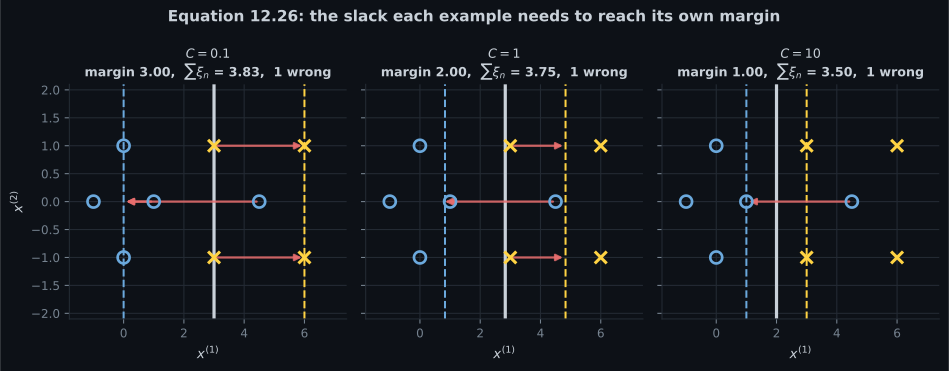
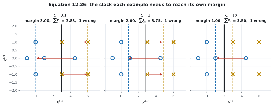
$\xi_n$ is how far example $n$ falls short of its own margin, measured in the units where the margin is $1$. Three regimes, and the book names only two of them:

$\xi_n$	where the example is
$\xi_n = 0$	correctly classified, at or beyond its margin — it costs nothing
$0 < \xi_n \leq 1$	correct side of the hyperplane, but inside the margin
$\xi_n > 1$	wrong side of the hyperplane

$\xi_n = 1$ is exactly the boundary between the last two, because $\xi_n = 1 - y_n f(\mathbf{x}_n)$ at the optimum and $y_n f(\mathbf{x}_n) = 0$ means the example sits on the hyperplane.

figure Equation 12.26: the slack each example needs to reach its own margin matplotlib

The red arrow on each violating point is its ξ, drawn as the distance it would have to travel to reach its own margin. At C = 0.1 the margin is wide and three examples pay for it; at C = 10 the margin has shrunk to 1 and only the intruder pays.

C is the price of a violation

The data below is page 1202’s impossible case: the running example plus a negative point at $(4.5, 0)$, which is the average of $(3, 1)$ and $(6, -1)$ and therefore sits strictly inside the positive class’s convex hull. No hyperplane can classify it correctly. The hard margin problem has no answer; the soft margin problem always has one.

setup.py

import numpy as np
from scipy.optimize import minimize
 
X = np.array([[3.0,  1.0], [3.0, -1.0], [6.0,  1.0], [6.0, -1.0],
              [1.0,  0.0], [0.0,  1.0], [0.0, -1.0], [-1.0, 0.0]])
Y = np.array([ 1.0,  1.0,  1.0,  1.0,  -1.0, -1.0, -1.0, -1.0])
XB = np.vstack([X, [4.5, 0.0]])          # the intruder
YB = np.r_[Y, -1.0]
 
def pred(scores):
    """Section 12.1's rule: f(x) >= 0 is class +1, ties included."""
    return np.where(scores >= 0.0, 1.0, -1.0)
 
def solve(XX, YY, C, seed):
    n, d = XX.shape
    rg = np.random.default_rng(seed)
    v0 = np.r_[rg.normal(0, 1, d), rg.normal(0, 1),
               np.abs(rg.normal(1, 0.5, n))]
    return minimize(lambda v: 0.5 * v[:d] @ v[:d]
                    + C * np.maximum(v[d + 1:], 0.0).sum(), v0,
                    constraints=[
                        {"type": "ineq",
                         "fun": lambda v: YY * (XX @ v[:d] + v[d]) - 1 + v[d + 1:]},
                        {"type": "ineq", "fun": lambda v: v[d + 1:]}],
                    method="SLSQP", options={"maxiter": 20000, "ftol": 1e-13})
 
def best(XX, YY, C, tries=30):
    out, bv = None, np.inf
    d = XX.shape[1]
    for s in range(tries):
        r = solve(XX, YY, C, s)
        if not r.success:
            continue
        w, b = r.x[:d], r.x[d]
        xi = np.maximum(0.0, 1 - YY * (XX @ w + b))   # the tight slack
        val = 0.5 * w @ w + C * xi.sum()
        if val < bv - 1e-12:
            bv, out = val, (w.copy(), float(b), xi)
    return out

the_c_sweep.py

print(f"{'C':>9} {'margin':>9} {'sum xi':>9} {'xi>0':>6} {'xi>1':>6} "
      f"{'wrong':>6} {'0.5||w||^2':>12} {'objective':>12}")
for C in (0.01, 0.1, 0.5, 1.0, 2.0, 10.0, 100.0, 1000.0):
    w, b, xi = best(XB, YB, C)
    nw = np.linalg.norm(w)
    print(f"{C:>9.2f} {1/nw:>9.4f} {xi.sum():>9.4f} "
          f"{int((xi > 1e-6).sum()):>6} {int((xi > 1 + 1e-6).sum()):>6} "
          f"{int((pred(XB @ w + b) != YB).sum()):>6} "
          f"{0.5*nw**2:>12.4f} {0.5*nw**2 + C*xi.sum():>12.4f}")

text

        C    margin    sum xi   xi>0   xi>1  wrong   0.5||w||^2    objective
     0.01    8.0000    6.4375      8      4      4       0.0078       0.0722
     0.10    3.0000    3.8333      4      1      1       0.0556       0.4389
     0.50    3.0000    3.8333      4      1      1       0.0556       1.9722
     1.00    2.0000    3.7500      4      1      1       0.1250       3.8750
     2.00    1.0000    3.5000      1      1      1       0.5000       7.5000
    10.00    1.0000    3.5000      1      1      1       0.5000      35.5000
   100.00    1.0000    3.5000      1      1      1       0.5000     350.5000
  1000.00    1.0000    3.5000      1      1      1       0.5000    3500.5000

Read the xi>0 and xi>1 columns against each other. At $C = 0.01$ every one of the nine examples is paying slack and four are on the wrong side; at $C = 10$ only the intruder pays anything at all. The book’s phrase “within the margin or even on the wrong side” covers two populations that move independently, and the count of violated margins is not the count of errors.

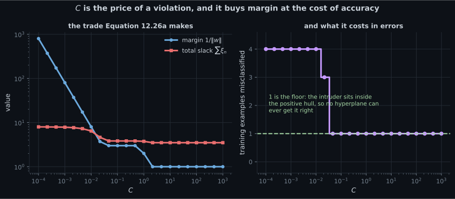
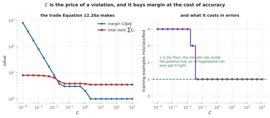
One training error is the floor, not a failure. The intruder is inside the positive hull, so no hyperplane of any kind gets it right. What $C$ buys above $C = 2$ is nothing: the solution has already stopped moving.

figure C is the price of a violation, and it buys margin at the cost of accuracy matplotlib

Both curves flatten above C ≈ 2. Past that point the constraint set is already satisfied as tightly as it can be and raising C only scales the objective — the last three rows of the table differ by a factor of ten in objective and not at all in solution.

The two limits

As $C \to \infty$ the slack becomes infinitely expensive, so on separable data the solver is forced back to the hard margin answer:

c_to_infinity.py

W_STAR, B_STAR = np.array([1.0, 0.0]), -2.0
print(f"{'C':>9} {'margin':>11} {'sum xi':>11} {'||w - w*||':>12} {'|b - b*|':>11}")
for C in (0.1, 0.5, 1.0, 5.0, 50.0, 500.0, 5000.0):
    w, b, xi = best(X, Y, C)               # the SEPARABLE running example
    print(f"{C:>9.1f} {1/np.linalg.norm(w):>11.6f} {xi.sum():>11.3e} "
          f"{np.linalg.norm(w - W_STAR):>12.3e} {abs(b - B_STAR):>11.3e}")

text

        C      margin      sum xi   ||w - w*||    |b - b*|
      0.1    2.000000   1.500e+00    5.000e-01   1.000e+00
      0.5    1.000000   2.139e-08    1.069e-08   3.208e-08
      1.0    1.000000   1.332e-15    5.334e-16   0.000e+00
      5.0    1.000000   6.217e-14    3.900e-15   2.043e-14
     50.0    1.000000   3.997e-15    4.415e-15   1.110e-14
    500.0    1.000000   0.000e+00    6.736e-13   7.665e-13
   5000.0    1.000000   0.000e+00    1.415e-15   2.220e-15

It does not take a large $C$ — by $C = 1$ the recovery is exact, and $|b - b^*|$ is literally zero. On separable data the hard margin solution is already feasible with zero slack, so any $C$ above a threshold reproduces it and there is nothing further to gain.

As $C \to 0$ the opposite happens: slack is free, weight is not, and the model gives up.

text

        C       ||w||      margin     sum xi  wrong
    1e-04    0.001250    800.0057     7.9844      4
    1e-03    0.012500     80.0001     7.8438      4
    1e-02    0.125000      8.0000     6.4375      4
    1e-01    0.333333      3.0000     3.8333      1
    2e-01    0.333333      3.0000     3.8333      1

$\lVert\mathbf{w}\rVert$ falls in proportion to $C$ and the margin balloons to $800$ — a “margin” that contains the entire dataset and means nothing. At $C = 0$ exactly, the optimum is $\mathbf{w} = \mathbf{0}$ and the classifier is constant. So $C$ is not a free knob at one end: it is a regularisation parameter and the book names it so, with the warning that its direction is the reverse of the usual convention — “a large value of $C$ implies low regularization”, because $C$ multiplies the error term rather than the regulariser.

At small C the boundary runs exactly through training points

Two rows of that sweep deserve a second look. At $C = 0.05$ and $C = 0.1$ the fitted parameters agree to fifteen decimal places, and the error count differs:

text

  C = 0.05:  w = [0.33333333 0.0]  b = -1.000000000000000
     f at (3, 1) and (3, -1) : +1.221e-15, -1.332e-15
     predicted labels there  : +1, -1   (true +1, +1)      ->  2 wrong
  C = 0.10:  w = [0.33333333 -0.0]  b = -0.999999999999994
     f at (3, 1) and (3, -1) : +3.553e-15, +7.105e-15
     predicted labels there  : +1, +1   (true +1, +1)      ->  1 wrong

The optimal boundary passes exactly through two training points, so which side they fall on is decided by the sign of a quantity that is zero up to rounding. Page 1201 found the same seam from the other direction: Equations 12.5, 12.6 and 12.7 disagree precisely on the hyperplane, and nowhere else.

The practical reading is that a reported training-error count is not a continuous function of $C$, and near a degenerate optimum it is not reproducible either.

The remark about b, which is not a remark

The book adds, in small type:

In the formulation of the soft margin SVM (12.26a) $\mathbf{w}$ is regularized, but $b$ is not regularized. We can see this by observing that the regularization term does not contain $b$. The unregularized term $b$ complicates theoretical analysis and decreases computational efficiency.

That reads as a minor inconvenience. It is the opposite — leaving $b$ out is what makes the method invariant to where you put the origin. Shift every example by a vector $\mathbf{t}$ and the pair $(\mathbf{w}, b - \langle\mathbf{w},\mathbf{t}\rangle)$ is feasible with the same slacks and the same $\tfrac12\lVert\mathbf{w}\rVert^2$, so the optimal value cannot change. Measured, with $\mathbf{t} = (10, 0)$:

$C$	$b$ penalised	$\lVert\mathbf{w}_{\text{new}} - \mathbf{w}_{\text{old}}\rVert$	$\lvert b_{\text{new}} - (b_{\text{old}} - \langle\mathbf{w},\mathbf{t}\rangle)\rvert$	change in objective
$0.1$	no	$1.993\times10^{-15}$	$7.105\times10^{-15}$	$9.437\times10^{-16}$
$0.1$	yes	$1.450\times10^{-1}$	$2.320$	$2.272\times10^{-1}$
$1.0$	no	$1.039\times10^{-8}$	$9.662\times10^{-3}$	$8.882\times10^{-16}$
$1.0$	yes	$3.619\times10^{-1}$	$4.790$	$3.673$
$10.0$	no	$9.812\times10^{-15}$	$1.332\times10^{-13}$	$9.948\times10^{-14}$
$10.0$	yes	$4.667\times10^{-1}$	$5.067$	$\mathbf{10.48}$

With $b$ free the objective value is unchanged to machine precision at every $C$, and $\mathbf{w}$ does not move. Add $\tfrac12 b^2$ to the objective and translating the data changes the answer — at $C = 10$ the optimal value moves by $10.48$ and $\lVert\mathbf{w}\rVert$ drops from $1.000000$ to $0.800000$. The penalised model has been told that a boundary near the origin is cheaper, and the origin is wherever somebody happened to put it.

One row where the parameters moved and the value did not

At $C = 1$ with $b$ free, $\lVert\mathbf{w}_{\text{new}} - \mathbf{w}_{\text{old}}\rVert = 1.039\times10^{-8}$ and the intercept is off by $9.662\times10^{-3}$ — far above the $10^{-15}$ of its neighbours. The objective gap is still $8.882\times10^{-16}$.

That is the signature of a non-unique optimum: at $C = 1$ the optimal set has a flat face, and the solver lands at different points of it on the shifted and unshifted problems. Both are correct answers. The invariance claim is about the optimal value and the classifier, and it holds exactly; the parameters are pinned only when the optimum is a single point.

pch.quizTag Check your understanding

1. A On the wrong side of the hyperplane B Exactly on the margin C On the correct side of the hyperplane but inside the margin — since xi = 1 - y f(x), a value below 1 means y f(x) is still positive D Correctly classified and beyond its margin
   pch.quizShowAnswer

   C — On the correct side of the hyperplane but inside the margin — since xi = 1 - y f(x), a value below 1 means y f(x) is still positive

2. A Only as C tends to infinity B By C = 1, where |b - b*| is exactly zero — the hard margin solution is already feasible with zero slack, so no further increase changes anything C Never, because slack is always positive D At C = 0
   pch.quizShowAnswer

   B — By C = 1, where |b - b*| is exactly zero — the hard margin solution is already feasible with zero slack, so no further increase changes anything

3. A Yes, a larger margin generalises better B No — the norm of w collapses in proportion to C, so the 'margin' 1/||w|| balloons while containing the whole dataset. At C = 0 exactly the optimum is w = 0 and the classifier is constant C Yes, because the total slack also falls D It depends on the dimension
   pch.quizShowAnswer

   B — No — the norm of w collapses in proportion to C, so the 'margin' 1/||w|| balloons while containing the whole dataset. At C = 0 exactly the optimum is w = 0 and the classifier is constant

4. A To simplify the theoretical analysis B Because b is always small C Because penalising b would make the solution depend on where the origin sits — measured, shifting the data by (10, 0) leaves the objective unchanged to 1e-15 with b free, and changes it by 10.48 with b penalised D Because b does not affect the margin
   pch.quizShowAnswer

   C — Because penalising b would make the solution depend on where the origin sits — measured, shifting the data by (10, 0) leaves the objective unchanged to 1e-15 with b free, and changes it by 10.48 with b penalised

Exercises

Exercise 1 – Classify the slack into three regimes

pch.exerciseTag pch.exerciseTitle

Exercise 2 – Recover the hard margin by raising C

pch.exerciseTag pch.exerciseTitle

Exercise 3 – Translate the data and see what moves

pch.exerciseTag pch.exerciseTitle

Recall card

• Real data is not separable, and page 1203’s hard margin problem simply has no answer on it. One negative point inside the positive class’s convex hull is enough.
• Section 12.2.4’s repair is one slack variable per example, subtracted from that example’s margin requirement and charged for in the objective.
• The slack splits into three regimes, and the book names two. Zero means the example costs nothing, between zero and one means inside the margin, above one means on the wrong side — because xi equals one exactly when the example sits on the hyperplane.
• The count of violated margins is not the count of errors. At C = 0.01 all nine examples pay slack and four are wrong; at C = 10 only one pays and one is wrong.
• C is the price of a violation, and a large C means low regularisation — the reverse of the usual convention, because C multiplies the error term rather than the regulariser.
• Above C = 2 on this data the solution stops moving entirely. The objective grows by a factor of ten across the last three rows and the parameters do not change at all.
• On separable data any large enough C recovers the hard margin exactly — by C = 1 the intercept matches to zero and the weights to 5.3e-16.
• As C tends to zero the weights collapse in proportion to it and the margin balloons to 800 while containing the whole dataset. At C = 0 the optimum is the constant classifier.
• Near a degenerate optimum the training-error count is not reproducible. At C = 0.05 the boundary runs exactly through two training points and their labels are decided by a quantity of size 1e-15.
• Leaving b out of the regulariser is what makes the method invariant to translating the data. Shifting by ten leaves the objective unchanged to 1e-15; penalising b changes it by 10.48 and shrinks the weights from 1.0 to 0.8.
• The origin is wherever somebody put it, and a model that prefers boundaries near it is answering a question about the coordinate system.

Next: The Hinge Loss — §12.2.5, the same optimisation problem written without any constraints at all.