The Hinge Loss

Page 1204 derived the soft margin SVM from geometry: draw a margin, let points fall short of it, charge for the shortfall. Section 12.2.5 derives the same problem from a different starting point — pick a loss function and minimise it, the programme of empirical risk minimisation in §8.2.

The hypothesis class is unchanged, $f(\mathbf{x}) = \langle\mathbf{w},\mathbf{x}\rangle + b$ (Equation 12.27). The only question is what to charge for a mistake.

The loss you want, and why you cannot have it

The natural loss counts mismatches — zero if the prediction is right, one if it is wrong. The book introduces it as the zero-one loss and immediately sets it aside: “the zero-one loss results in a combinatorial optimization problem for finding the best parameters $\mathbf{w}, b$.”

It is worth seeing how bad that is, because it is what everything else is compared against. In $\mathbb{R}^2$ the minimum-error linear classifier can be found exactly, by enumeration: the optimum is always attained at a direction normal to some pair of points, with the threshold scanned across sorted projections.

the_zero_one_optimum.py

import itertools
import numpy as np
 
X = np.array([[3.0,  1.0], [3.0, -1.0], [6.0,  1.0], [6.0, -1.0],
              [1.0,  0.0], [0.0,  1.0], [0.0, -1.0], [-1.0, 0.0]])
Y = np.array([ 1.0,  1.0,  1.0,  1.0,  -1.0, -1.0, -1.0, -1.0])
XB = np.vstack([X, [4.5, 0.0]])          # page 1204's non-separable case
YB = np.r_[Y, -1.0]
 
def pred(s):
    return np.where(s >= 0.0, 1.0, -1.0)
 
def min_zero_one(XX, YY):
    dirs = []
    for i, j in itertools.combinations(range(len(XX)), 2):
        dv = XX[i] - XX[j]
        dirs += [np.array([-dv[1], dv[0]]), dv.copy()]
    dirs += [np.array([np.cos(t), np.sin(t)])
             for t in np.linspace(0, 2 * np.pi, 720, endpoint=False)]
    bestE, bestP = len(XX) + 1, None
    for w in dirs:
        if np.linalg.norm(w) < 1e-12:
            continue
        w = w / np.linalg.norm(w)
        p = XX @ w
        cuts = np.unique(np.r_[p - 1e-7, p + 1e-7,
                               (p[:, None] + p[None, :]).ravel() / 2])
        for c in cuts:
            for sgn in (1.0, -1.0):
                ww, bb = sgn * w, -sgn * c
                e = int((pred(XX @ ww + bb) != YY).sum())
                if e < bestE:
                    bestE, bestP = e, (ww, bb)
    return bestE, bestP
 
e01, (w01, b01) = min_zero_one(XB, YB)
print(f"minimum achievable training errors : {e01}")
print(f"attained by w = {np.round(w01, 6)}, b = {b01:.6f}")

text

minimum achievable training errors : 1
attained by w = [ 1. -0.], b = -3.000000

That took a search over roughly $3{,}000$ directions and $80$ thresholds each. In $D$ dimensions the same enumeration is over $O(N^D)$ candidate hyperplanes — which is precisely why the chapter needs a surrogate.

The hinge loss

$$\ell(t) = \max\{0,\ 1 - t\} \qquad\text{where}\qquad t = y f(\mathbf{x}) = y(\langle\mathbf{w},\mathbf{x}\rangle + b) \qquad \text{(12.28)}$$

or, written as the two linear pieces §12.5 will differentiate,

$$\ell(t) = \begin{cases} 0 & \text{if } t \geq 1\\ 1 - t & \text{if } t < 1\end{cases} \qquad \text{(12.29)}$$

The book also gives the hard margin’s loss for comparison — $0$ if $t \geq 1$ and $\infty$ otherwise, Equation 12.30, “never allowing any examples inside the margin.”

The regularised objective is then completely unconstrained:

$$\min_{\mathbf{w}, b}\ \underbrace{\tfrac12\lVert\mathbf{w}\rVert^2}_{\text{regularizer}} + C\sum_{n=1}^{N}\underbrace{\max\{0,\ 1 - y_n(\langle\mathbf{w},\mathbf{x}_n\rangle + b)\}}_{\text{error term}} \qquad \text{(12.31)}$$

Margin maximisation has become regularisation. The term that came from geometry on page 1203 is now the thing that keeps the weights small, and the book says so explicitly.

figure The hinge bounds the zero-one loss from above, and stops charging once you are right matplotlib

Left, the shaded band is what the surrogate over-charges — largest just above t = 0, where it approaches 1. Right, the squared loss is the only one of the three that rises as the prediction becomes more confidently correct.

It is the same problem as Equation 12.26

The book’s argument is that a hinge can be traded for a slack variable and two constraints:

$$\min_t\ \max\{0,\ 1-t\} \qquad\text{is equivalent to}\qquad \min_{\xi, t}\ \xi \ \text{ subject to }\ \xi \geq 0,\ \xi \geq 1 - t \qquad \text{(12.32), (12.33)}$$

Substituting that into 12.31 and rearranging gives exactly 12.26. The content is that the slack variables were never independent unknowns — at the optimum the binding constraint pins $\xi = \max\{0, 1-t\}$, which is the hinge again.

same_problem.py

print(f"{'C':>8} {'objective 12.26':>17} {'objective 12.31':>17} {'gap':>11}")
for C in (0.1, 0.5, 1.0, 2.0, 10.0):
    _, fc = best_constrained(XB, YB, C)      # N + D + 1 vars, 2N constraints
    _, fu = best_unconstrained(XB, YB, C)    # D + 1 vars, no constraints
    print(f"{C:>8.2f} {fc:>17.10f} {fu:>17.10f} {abs(fc - fu):>11.2e}")

text

       C   objective 12.26   objective 12.31         gap
    0.10      0.4388888889      0.4388888889    4.45e-13
    0.50      1.9722222222      1.9722222222    5.12e-13
    1.00      3.8750000000      3.8750000000    4.44e-16
    2.00      7.5000000000      7.5000000000    2.73e-13
   10.00     35.5000000000     35.5000000000    4.90e-13

Ten significant figures, on a problem with $12$ variables and $18$ constraints versus one with $3$ variables and none. Checking the slacks at the fitted optimum ($C = 1$) against $\max\{0, 1 - y_n f(\mathbf{x}_n)\}$:

text

[0.91584099 0.91584096 0. 0. 0.08415903 0. 0. 0. 1.83415902]
sum = 3.75000000

which is page 1204’s $\sum\xi_n = 3.7500$ exactly. Note that the ninth entry — the intruder at $(4.5, 0)$ — exceeds $1$, confirming it is on the wrong side, while the two entries near $0.916$ are examples inside the margin but correctly classified.

Equal values, and sometimes unequal parameters

The objective values above agree to $10^{-13}$ or better. At $C = 1$ the parameters returned by the two solvers differ by $8.70\times10^{-2}$ in $b$ while the objective gap is $4.44\times10^{-16}$.

That is page 1204’s degenerate optimum again: at $C = 1$ the optimal set has a flat face and the two solvers land at different points of it. Both answers are correct. Whenever a soft-margin fit is reported, it is the objective value that is well defined, and the parameters only when the optimum is a single point.

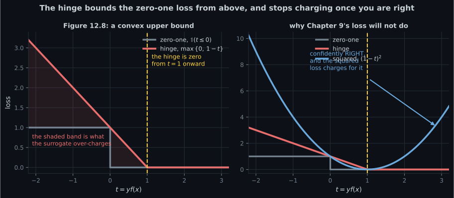
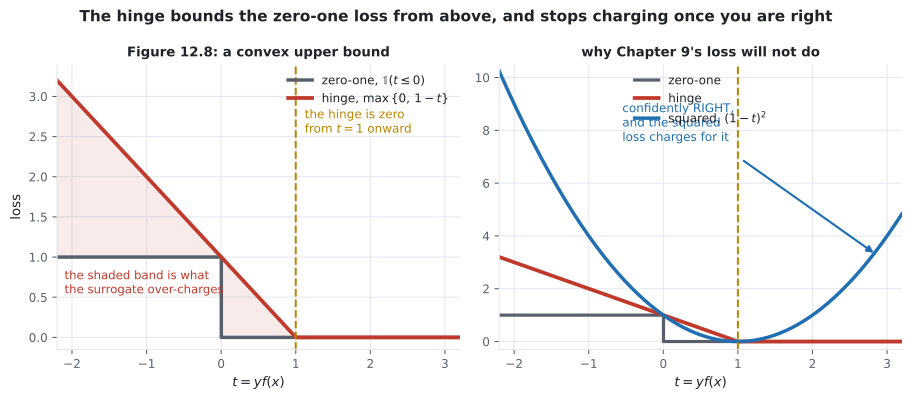
How much does the surrogate cost?

The hinge is a convex upper bound on the zero-one loss, which is what makes minimising it useful: drive the bound down and the thing it bounds comes down too.

$t = y f(\mathbf{x})$	zero-one	hinge	gap
$-2.00$	$1$	$3.00$	$2.00$
$-0.50$	$1$	$1.50$	$0.50$
$0.00$	$1$	$1.00$	$\mathbf{0.00}$
$0.50$	$0$	$0.50$	$0.50$
$1.00$	$0$	$0.00$	$\mathbf{0.00}$
$3.00$	$0$	$0.00$	$0.00$

Checked on a two-million-point grid over $[-50, 50]$, the hinge is never below the zero-one loss. The bound is tight in two places — at $t = 0$ and for all $t \geq 1$ — and the gap grows without bound as $t \to -\infty$, where it equals $-t$: a badly misclassified example is charged far more than the $1$ it costs in errors.

The interesting region is the other one. On $0 < t < 1$ the example is correctly classified and the hinge still charges it $1 - t$, a penalty approaching $1$ as $t \to 0^+$ and never attaining it:

text

t = 1e-03 : gap = 0.999000000000
t = 1e-06 : gap = 0.999999000000
t = 1e-09 : gap = 0.999999999000

And the surrogate’s practical cost, against the exact zero-one optimum computed above:

$C$	errors from the hinge fit	zero-one optimum	excess
$0.01$	$4$	$1$	$3$
$1.00$	$1$	$1$	$\mathbf{0}$
$10.00$	$1$	$1$	$\mathbf{0}$
$100.00$	$1$	$1$	$\mathbf{0}$

On this data the surrogate costs nothing once $C$ is large enough. That is not a theorem — the hinge minimiser and the zero-one minimiser are different objectives and can disagree — but it is the usual situation, and it is why the substitution is worth making.

Why not Chapter 9’s squared loss?

The book dismisses it in one sentence: “the squared loss that is used for regression (9.10b) is not suitable for binary classification.” What goes wrong is specific and worth seeing.

$t = y f(\mathbf{x})$	hinge	squared $(1-t)^2$	what the example is
$-2.0$	$3.00$	$9.00$	badly wrong
$0.5$	$0.50$	$0.25$	right, inside the margin
$1.0$	$0.00$	$0.00$	right, on the margin
$3.0$	$0.00$	$4.00$	right, confident
$10.0$	$0.00$	$\mathbf{81.00}$	right, very confident

The squared loss charges $81$ for being confidently right and $9$ for being wrong. It has no notion of a correct side: it wants $f(\mathbf{x})$ to equal $y$, and treats overshooting as an error of the same kind as being on the wrong side altogether.

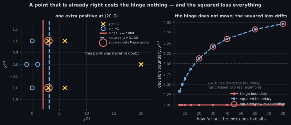
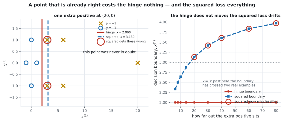
That is not a curiosity. Add one extra positive example at $(D, 0)$ — correctly labelled, on its own side, in no doubt at all — and push it away:

text

  outlier at   hinge boundary  hinge err   squared boundary  squared err
      (6, 0)         2.000000          0           2.330729            0
     (10, 0)         2.000000          0           2.640625            0
     (20, 0)         2.000000          0           3.129934            2
     (40, 0)         2.000000          0           3.602371            2
     (80, 0)         2.000000          0           3.968750            2

The hinge boundary does not move at all — $2.000000$ in every row. Once the outlier is beyond its margin it contributes exactly zero, and the fit is decided entirely by the points near the boundary. The squared-loss boundary drifts from $2.33$ to $3.97$, crosses $x = 3$, and starts misclassifying two examples that were never in doubt.

At the hinge’s own solution the outlier’s squared loss is $5929$ while its hinge loss is $0$. A squared-loss fit spends its whole budget bringing that number down.

figure A point that is already right costs the hinge nothing — and the squared loss everything matplotlib

The flat red line is the point. The hinge's insensitivity to examples beyond the margin is the same property that makes the dual of page 1206 sparse: most examples contribute nothing to the answer.

That insensitivity is not a side effect. It is the property that makes page 1206’s dual sparse — examples beyond the margin have zero loss, zero gradient, and, it will turn out, zero Lagrange multiplier.

pch.quizTag Check your understanding

1. A Because it is not an upper bound B Because it gives the wrong answer C Because it is piecewise constant, so it has no useful gradient and the optimisation becomes combinatorial — in D dimensions the exact search is over O(N^D) candidate hyperplanes D Because it requires the data to be separable
   pch.quizShowAnswer

   C — Because it is piecewise constant, so it has no useful gradient and the optimisation becomes combinatorial — in D dimensions the exact search is over O(N^D) candidate hyperplanes

2. A That the slack variables add expressive power B That the slack variables were never independent unknowns — at the optimum the binding constraint pins xi to max(0, 1-t), which is the hinge again C That the problem is non-convex D That the hinge loss is differentiable
   pch.quizShowAnswer

   B — That the slack variables were never independent unknowns — at the optimum the binding constraint pins xi to max(0, 1-t), which is the hinge again

3. A Equal everywhere; the gap is always zero B Equal at t = 0 and for all t >= 1; the gap grows without bound as t tends to minus infinity, where it equals -t C Equal only at t = 1; the gap grows as t tends to plus infinity D Equal for t < 0; the gap grows inside the margin
   pch.quizShowAnswer

   B — Equal at t = 0 and for all t >= 1; the gap grows without bound as t tends to minus infinity, where it equals -t

4. A It does not; the charge is negligible B Because it is what pulls the boundary away from correctly classified points that sit too close to it — the penalty approaches 1 as t tends to zero from above, the same size as the charge for an outright error C Because it makes the loss non-convex D Because it means the hinge is not an upper bound there
   pch.quizShowAnswer

   B — Because it is what pulls the boundary away from correctly classified points that sit too close to it — the penalty approaches 1 as t tends to zero from above, the same size as the charge for an outright error

5. A The hinge loss ignores positive examples B The squared loss is not convex C Once an example is beyond its margin the hinge charges exactly zero for it, so it stops influencing the fit; the squared loss charges (1 - f)^2, which grows without bound as the example moves away D The hinge boundary is fixed by the regulariser
   pch.quizShowAnswer

   C — Once an example is beyond its margin the hinge charges exactly zero for it, so it stops influencing the fit; the squared loss charges (1 - f)^2, which grows without bound as the example moves away

Exercises

Exercise 1 – Show the hinge bounds the zero-one loss

pch.exerciseTag pch.exerciseTitle

Exercise 2 – Solve 12.31 with no constraints at all

pch.exerciseTag pch.exerciseTitle

Exercise 3 – Drag the boundary with a squared loss

pch.exerciseTag pch.exerciseTitle

Recall card

• Section 12.2.5 rebuilds the soft margin SVM from a loss function instead of from geometry, following the empirical risk minimisation programme of Section 8.2, and arrives at the same problem.
• The loss you actually want is the zero-one loss, and minimising it is combinatorial — the exact search in D dimensions is over order N to the D candidate hyperplanes.
• In two dimensions it can still be enumerated. On the non-separable running example the true minimum is one error, attained at w equal to (1, 0) and b equal to minus three.
• The hinge loss is a convex upper bound on the zero-one loss, exactly tight at t equals zero and for every t at or beyond one, and growing without bound as t goes to minus infinity — so a badly misclassified point is over-charged without limit.
• On the interval where the prediction is right but inside the margin, the hinge still charges up to one — almost as much as an outright error. That charge is the margin, written as a loss.
• So minimising the bound pushes the error rate down, and unlike the thing it bounds, the bound is convex.
• Equation 12.31 has no constraints at all — D plus one variables against Equation 12.26’s N plus D plus one variables and two N constraints — and the two agree to ten significant figures.
• The slack variables were never independent unknowns. At the optimum the binding constraint pins each one to the hinge value, which is what Equations 12.32 and 12.33 say.
• Margin maximisation is regularisation. The squared-norm term that came from geometry on page 1203 is the regulariser here, and the book names it as such.
• The surrogate cost nothing on this data once C was large enough: one training error, matching the exact zero-one optimum.
• Chapter 9’s squared loss charges 81 for being confidently right and 9 for being wrong. It wants f to equal y, and has no notion of a correct side.
• Measured, that breaks the classifier. A correctly labelled point pushed from 6 to 80 leaves the hinge boundary at exactly 2.000000 and drags the squared-loss boundary from 2.33 to 3.97, misclassifying two examples that were never in doubt.
• The hinge’s blindness to examples beyond the margin is not a side effect. It is what makes the dual of the next page sparse.

Next: The Dual Support Vector Machine — §12.3.1, where the same problem is rewritten in terms of the examples rather than the features.