Updating the Mixture Weights

Two updates down, one to go — and this one is different. The means and covariances were unconstrained, so setting a derivative to zero was enough. The weights have to stay on a simplex, so §11.2.4 is the only place in the chapter that reaches for Chapter 7.

What you’ll learn

• Theorem 11.3, Equation 11.42, and Example 11.5 reproduced: $\tfrac13 \to 0.293890,\ 0.287001,\ 0.419109$, which round to the book’s $0.29$, $0.29$ and $0.42$.
• The Lagrangian of Equations 11.43–11.48, and $\lambda$ solved from each component separately: exactly $-7 = -N$, all three agreeing to $0.0$.
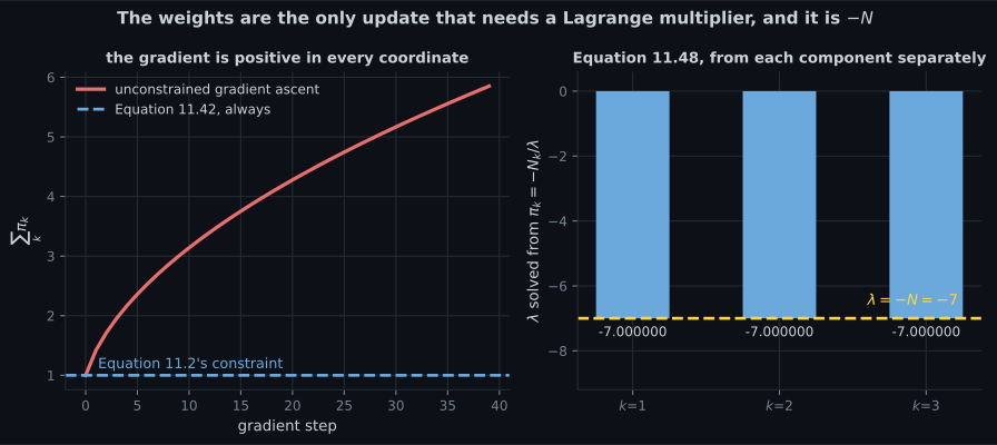
• Why the constraint is not a formality: the gradient of $L$ in $\boldsymbol\pi$ is strictly positive in every coordinate, so unconstrained ascent sends every weight to infinity.
• Why no projection onto the simplex is ever needed afterwards: measured over $50{,}000$ random responsibility matrices, the weights sum to $1$ to $2.2\times10^{-16}$ and none ever leaves $[0,1]$.
• What this update alone is worth: $+0.137132$ nats, the smallest of the three.
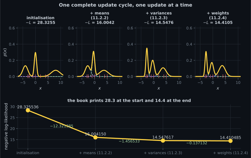
• The complete cycle, matching the book’s own figures: negative log-likelihood $\mathbf{28.325536 \to 14.410485}$, printed as $28.3 \to 14.4$.
• And the one structural thing that separates this update from the other two: it never looks at $\mathbf{x}$.

Intuition: counting, not averaging

The first two updates asked where and how wide. This one asks how much, and the answer is the one you would write down without any calculus: the share of the data each component ended up owning.

$N_k$ is that share — page 1103’s effective count. Divide by $N$ and you have a proportion. The Lagrange multiplier’s entire job is to confirm that the obvious answer is also the optimal one, and the multiplier it produces, $-N$, is exactly the normalising constant you would have divided by anyway.

diagram Why this one needs Chapter 7 and the others do not mermaid

  flowchart TD
  A["mu_k: unconstrained in R^D"] --> B["set dL/dmu = 0
Theorem 11.1"]
  C["Sigma_k: must be PSD"] --> D["set dL/dSigma = 0
Theorem 11.2 -- PSD comes free"]
  E["pi_k: must lie on the simplex"] --> F["dL/dpi is positive everywhere
no interior stationary point"]
  F --> G["Lagrangian, Equation 11.43
lambda = -N"]
  G --> H["pi_k = N_k / N
Equation 11.42"]

§11.2.4 Theorem 11.3

Theorem 11.3 (Update of the GMM Mixture Weights). The mixture weights of the GMM are updated as

$$\pi_k^{\text{new}} = \frac{N_k}{N}, \qquad k = 1,\ldots,K \qquad \text{(11.42)}$$

The proof accounts for $\sum_k\pi_k = 1$ with a Lagrange multiplier:

$$\mathfrak{L} = L + \lambda\left(\sum_{k=1}^{K}\pi_k - 1\right) \qquad \text{(11.43a)}$$ $$\frac{\partial\mathfrak{L}}{\partial\pi_k} = \frac{1}{\pi_k}\underbrace{\sum_{n=1}^{N}\frac{\pi_k\mathcal{N}(\mathbf{x}_n\mid\boldsymbol\mu_k,\boldsymbol\Sigma_k)}{\sum_j\pi_j\mathcal{N}(\mathbf{x}_n\mid\boldsymbol\mu_j,\boldsymbol\Sigma_j)}}_{=\,N_k} + \lambda = \frac{N_k}{\pi_k} + \lambda \qquad \text{(11.44b)}$$

Setting both partials to zero gives $\pi_k = -N_k/\lambda$ and $\sum_k\pi_k = 1$, so $-\sum_k N_k/\lambda = 1$, and since $\sum_k N_k = N$:

$$\lambda = -N \qquad \text{(11.48)}$$

Measured, solving $\lambda = -N_k/\pi_k$ from each component independently:

	$\lambda$
from $k=1$	$-7.000000000000$
from $k=2$	$-7.000000000000$
from $k=3$	$-7.000000000000$
$-N$	$-7$

with a largest deviation of $0.0$, and Equation 11.44b’s stationarity condition $N_k/\pi_k + \lambda$ equal to $+0.0$ in every component.

$k$	$\pi_k$ before	$\pi_k$ after	the book	$N_k$
$1$	$0.333333$	$\mathbf{0.293890}$	$0.29$	$2.057228$
$2$	$0.333333$	$\mathbf{0.287001}$	$0.29$	$2.009008$
$3$	$0.333333$	$\mathbf{0.419109}$	$0.42$	$2.933763$

summing to $1.000000000000000$.

The constraint is doing real work

It is tempting to treat $\sum_k\pi_k = 1$ as bookkeeping — enforce it at the end and move on. It cannot be done that way, because there is no unconstrained optimum to enforce it on. From Equation 11.44a,

$$\frac{\partial L}{\partial\pi_k} = \sum_{n=1}^{N}\frac{\mathcal{N}(\mathbf{x}_n\mid\boldsymbol\mu_k,\boldsymbol\Sigma_k)}{\sum_j\pi_j\mathcal{N}(\mathbf{x}_n\mid\boldsymbol\mu_j,\boldsymbol\Sigma_j)} > 0$$

— a sum of positive terms, in every coordinate. Plain gradient ascent:

step	$\boldsymbol\pi$	$\sum_k\pi_k$
$0$	$0.3333,\ 0.3333,\ 0.3333$	$1.000000$
$1$	$0.4531,\ 0.4535,\ 0.5134$	$1.420000$
$2$	$0.5411,\ 0.5418,\ 0.6304$	$1.713336$
$6$	$0.7925,\ 0.7936,\ 0.9508$	$2.536943$

figure Without the constraint there is nothing to find; with it, the answer is a count matplotlib

Every unnormalised weight makes the likelihood larger, so the unconstrained problem has no maximum — the left panel simply climbs. On the right, lambda solved separately from each of the three components gives minus seven every time, which is minus N.

The multiplier is the normaliser

$\lambda = -N$ is not a coincidence of this dataset. The stationarity condition is $\pi_k = -N_k/\lambda$, so $\lambda$ is whatever makes the $N_k$ sum to one after division — and $\sum_k N_k = N$ by page 1103’s column-sum identity. The Lagrange multiplier turns out to be the normalising constant.

That is the cleanest possible outcome of a constrained optimisation: the constraint does not distort the answer, it only rescales it. Contrast page 1002’s Lagrangian, where the multiplier came out as an eigenvalue and carried real information.

And afterwards, the constraint never needs enforcing again

Because $\pi_k = N_k/N$ with $N_k \geq 0$ and $\sum_k N_k = N$:

$50{,}000$ random responsibility matrices, $K = 4$	value
worst $\lvert\sum_k\pi_k - 1\rvert$	$2.2\times10^{-16}$
weights falling outside $[0,1]$	$\mathbf{0}$

No clipping, no renormalisation, no projection. This is the same kind of structural guarantee page 1105 found for positive semi-definiteness — the update produces a valid object because of what it is, not because anything checks it afterwards.

One complete cycle

Applying all three updates in §11.3’s order, one at a time:

after	negative log-likelihood	gained
the initialisation	$28.325536$
$+$ means (§11.2.2)	$16.004150$	$12.321385$
$+$ variances (§11.2.3)	$14.547617$	$1.456533$
$+$ weights (§11.2.4)	$\mathbf{14.410485}$	$0.137132$

figure The book's 28.3 and 14.4, and the two steps in between matplotlib

The means do most of the work — 12.321385 of the 13.915051 nats gained — because the initialisation put them furthest from the data. The weights do the least, 0.137132, because with three roughly equal clusters there was not much to reallocate.

The order of the gains is not an accident of this example

The means moved the likelihood by $12.32$ nats, the variances by $1.46$, the weights by $0.14$ — a hundred-fold spread.

That ordering reflects how badly each parameter was initialised, not any intrinsic importance. The book chose $\mu = (-4, 0, 8)$ with data in $[-3, 5]$, so the means had the furthest to travel. Page 1104 measured the same thing from the other side: the first mean update moves by $4.295713$ and the second by $0.130775$.

What is general: the weights can only ever reallocate mass between components that already exist, so their update is bounded by how unequal the clusters are. With $K$ balanced clusters the weight update does almost nothing at all.

The only update that never sees the data

$\boldsymbol\mu_k$ and $\boldsymbol\Sigma_k$ are averages of $\mathbf{x}$. $\pi_k$ is a count. Holding the responsibility matrix fixed and permuting the data values:

data	$\boldsymbol\pi$
$-2.5,\ 2,\ -1,\ 0,\ 5,\ 4,\ -3$	$0.293890,\ 0.287001,\ 0.419109$
$-3,\ -2.5,\ 0,\ 5,\ 2,\ -1,\ 4$	$0.293890,\ 0.287001,\ 0.419109$
the original	$0.293890,\ 0.287001,\ 0.419109$

Identical, because Equation 11.42 reads only the column sums of $\mathbf{r}$. The data enters the weight update only through the responsibilities — which is exactly the structure §11.4.5 will formalise as the E-step supplying sufficient statistics to the M-step.

pch.quizTag Is the weight update clear?

1. Why does Section 11.2.4 need a Lagrange multiplier when Sections 11.2.2 and 11.2.3 do not?

   A Because the weights are scalars B Because the log-likelihood's gradient in pi is strictly positive in every coordinate, so there is no unconstrained stationary point to find C Because the weights can be negative D To make the derivation shorter
   pch.quizShowAnswer

   B — Because the log-likelihood's gradient in pi is strictly positive in every coordinate, so there is no unconstrained stationary point to find — Measured: plain gradient ascent takes the weights from summing to 1 to summing to 2.54 in six steps and keeps climbing. The means and covariances have genuine interior optima; the weights only have one once the simplex constraint is imposed.

2. What does the Lagrange multiplier come out to be?

   A An eigenvalue, as in Section 10.2 B Exactly minus N — it is the normalising constant, because the N_k already sum to N C Zero D It depends on the data
   pch.quizShowAnswer

   B — Exactly minus N — it is the normalising constant, because the N_k already sum to N — Solved independently from each of the three components it gives minus 7.000000000000 every time, to a deviation of 0.0. Contrast Section 10.2's Lagrangian, where the multiplier was an eigenvalue and carried real information; here the constraint only rescales.

3. After the update, how are the weights kept on the simplex?

   A By clipping them to [0, 1] B Nothing is needed — N_k over N is automatically non-negative and sums to one, because the responsibilities' rows sum to one C By renormalising at the end of each iteration D By a projection step
   pch.quizShowAnswer

   B — Nothing is needed — N_k over N is automatically non-negative and sums to one, because the responsibilities' rows sum to one — Measured over 50,000 random responsibility matrices with K = 4: the weights sum to 1 to 2.2e-16 and not one falls outside [0, 1]. The same kind of structural guarantee page 1105 found for positive semi-definiteness.

4. What is structurally different about the weight update compared to the other two?

   A Nothing B It never looks at the data values — only at the column sums of the responsibility matrix C It is not derived from the likelihood D It requires the covariances
   pch.quizShowAnswer

   B — It never looks at the data values — only at the column sums of the responsibility matrix — Permuting the data while holding the responsibilities fixed leaves the weights identical to six decimals. The means and covariances are averages of x; the weight is a count. Section 11.4.5 formalises this as the E-step passing sufficient statistics to the M-step.

Exercises

Exercise 1 – Reproduce Example 11.5, and solve for lambda

pch.exerciseTag pch.exerciseTitle

Exercise 2 – Try it without the constraint

pch.exerciseTag pch.exerciseTitle

Exercise 3 – The simplex takes care of itself

pch.exerciseTag pch.exerciseTitle

Exercise 4 – The complete cycle, and the book’s two numbers

pch.exerciseTag pch.exerciseTitle

Exercise 5 – The weights never see the data

pch.exerciseTag pch.exerciseTitle

Recall card

• Theorem 11.3: each weight becomes that component’s share of the data, its total responsibility divided by the number of points.
• This is the only update in the chapter that needs a Lagrange multiplier, because the weights must lie on a simplex and the other two parameters are unconstrained.
• The constraint is not bookkeeping. The log-likelihood’s gradient in the weights is strictly positive in every coordinate, so unconstrained ascent has nothing to converge to — measured, the weights’ sum reaches 2.54 in six steps and keeps climbing.
• The multiplier comes out as exactly minus N, solved independently from each component to a deviation of zero. It is the normalising constant, not new information.
• Contrast Section 10.2’s Lagrangian, where the multiplier was an eigenvalue and told you the variance retained.
• Afterwards the simplex looks after itself: over fifty thousand random responsibility matrices the weights sum to one to 2.2e-16 and never leave the unit interval.
• Example 11.5 reproduced: a third becomes 0.293890, 0.287001 and 0.419109, rounding to the book’s 0.29, 0.29 and 0.42.
• The complete cycle takes the negative log-likelihood from 28.325536 to 14.410485, which is the book’s 28.3 and 14.4.
• The means supply 12.32 of the 13.92 nats gained, the variances 1.46, the weights 0.14 — an ordering that reflects how badly each was initialised.
• But the weights can only ever reallocate mass between components that already exist, so with balanced clusters their update does almost nothing whatever the initialisation.
• And this is the only update that never reads the data values. Permuting the data with the responsibilities held fixed leaves the weights identical and moves every mean.

Next: The EM Algorithm — §11.3, which puts the three updates in a loop and states the guarantee that makes the loop worth running.