Functions, Limits, and Continuity

“A function” sounds like the least interesting item on a prerequisites list. It is on this one because Chapter 2 will ask whether a linear mapping is injective, surjective or bijective and use the answer to decide whether a matrix has an inverse — and Chapter 5 will differentiate things, which requires a limit, which requires knowing what a limit is.

Both are ten-minute ideas that get skipped and then quietly cost hours.

What you’ll learn

• Domain, codomain and image, and why the image is usually smaller than the codomain.
• Injective, surjective, bijective — and the exact sentence that connects them to matrix inverses.
• What a limit is, including the two-sided requirement that makes it fail.
• Continuity as “no jumps”, stated precisely enough to check.
• Why differentiable implies continuous but not the reverse, with ReLU as the example that matters.

Intuition: a function is a machine with a rule

A function is three things, not one: a set of allowed inputs, a set the outputs are drawn from, and a rule. The rule must give exactly one output for each input — that requirement is the whole definition, and everything else is bookkeeping about the two sets.

diagram Diagram mermaid

  flowchart LR
  D["domain
every allowed input"] -->|"rule f"| C["codomain
the set outputs are drawn from"]
  D -.-> I["image
the outputs actually produced"]
  I --> C
  C --> N["codomain minus image
values f never reaches"]

The gap between image and codomain is the part people skip, and it is exactly the gap that Chapter 2 turns into a statement about solvability. If $f(x) = x^2$ with domain and codomain both $\mathbb{R}$, the image is only $[0, \infty)$. Ask for an $x$ with $f(x) = -4$ and there is none — not because the arithmetic is hard, but because $-4$ is in the codomain and not in the image. Replace $f$ with a matrix and that is precisely the situation ”$\mathbf{A}\mathbf{x} = \mathbf{b}$ has no solution”.

The math

The three sets

$$f : \mathcal{D} \to \mathcal{C}, \qquad x \mapsto f(x)$$

• $\mathcal{D}$ is the domain: every input the function accepts.
• $\mathcal{C}$ is the codomain: the set the outputs live in.
• $\operatorname{Im}(f) = \{f(x) : x \in \mathcal{D}\} \subseteq \mathcal{C}$ is the image: the outputs actually achieved.

The book writes $\operatorname{Im}(\Phi)$ for the image of a linear mapping $\Phi$ and calls it the range or column space when $\Phi$ is a matrix. Same object, three names, and §2.7 uses all of them.

Injective, surjective, bijective

These three words are the reason this page exists.

$$\begin{aligned} f \text{ is \textbf{injective}} \quad&\Longleftrightarrow\quad f(x) = f(y) \implies x = y \\[2pt] f \text{ is \textbf{surjective}} \quad&\Longleftrightarrow\quad \operatorname{Im}(f) = \mathcal{C} \\[2pt] f \text{ is \textbf{bijective}} \quad&\Longleftrightarrow\quad \text{both} \end{aligned}$$

In words a reader can hold on to:

property	plain English	what fails without it
injective	different inputs give different outputs — nothing collapses	you cannot undo $f$: two inputs share an output, so “which one was it?” has no answer
surjective	every value in the codomain is hit by something	some targets are unreachable, so “solve $f(x) = b$” can fail
bijective	a perfect pairing, both ways	nothing; a bijection has a genuine inverse $f^{-1}$

An inverse exists exactly when $f$ is bijective. That is the sentence. Chapter 2 then says: a square matrix is invertible exactly when the linear mapping it defines is bijective, which happens exactly when its columns are linearly independent, which happens exactly when its rank is full, which happens exactly when its determinant is nonzero. Five statements, one condition — and the chain starts here.

Injective means the kernel is trivial

For a linear map there is a shortcut, and §2.7 leans on it hard. Linearity gives $f(x) = f(y) \iff f(x - y) = \mathbf{0}$, so $f$ is injective exactly when the only vector it sends to zero is zero itself:

$$f \text{ injective} \quad\Longleftrightarrow\quad \ker(f) = \{\mathbf{0}\}$$

Checking injectivity for a general function means comparing every pair of inputs. For a linear one it means solving a single homogeneous system. That collapse from “all pairs” to “one system” is what makes linear algebra tractable, and it is worth noticing the first time you see it.

Limits

$$\lim_{x \to a} f(x) = L$$

reads: as $x$ gets arbitrarily close to $a$, $f(x)$ gets arbitrarily close to $L$. Two things this does not say, both of which matter:

• It says nothing about $f(a)$. The function need not even be defined at $a$.
• It requires the same $L$ from both sides.

The two-sided requirement is where limits fail:

$$\lim_{x \to a^-} f(x) \;=\; \lim_{x \to a^+} f(x) \;=\; L \quad\Longleftrightarrow\quad \lim_{x \to a} f(x) = L$$

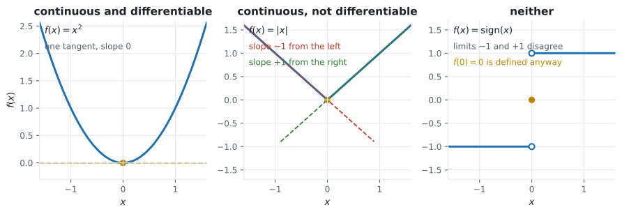
For $f(x) = \operatorname{sign}(x)$ the left limit at $0$ is $-1$ and the right limit is $+1$. They disagree, so $\lim_{x\to 0} f(x)$ does not exist — regardless of the fact that $f(0) = 0$ is perfectly well defined.

The canonical example of a limit that exists where the function does not is

$$\lim_{x \to 0} \frac{\sin x}{x} = 1,$$

which is undefined at $0$ but has a perfectly good limit approaching it. Every derivative is a limit of this kind: a quotient that is $0/0$ at the point of interest and has a limit anyway.

Continuity

$f$ is continuous at $a$ when all three of these hold:

1. $f(a)$ is defined,
2. $\lim_{x\to a} f(x)$ exists,
3. they are equal: $\lim_{x\to a} f(x) = f(a)$.

Continuous on an interval means continuous at every point of it. Informally: you can draw the graph without lifting the pen. All three conditions are needed — a function can satisfy any two and fail the third, which is why the definition is a list rather than a sentence.

Differentiability

$$f'(a) \;=\; \lim_{h \to 0} \frac{f(a + h) - f(a)}{h}$$

$f$ is differentiable at $a$ when that limit exists. Because it is a two-sided limit, the slope approaching from the left must match the slope approaching from the right.

$$\text{differentiable at } a \;\Longrightarrow\; \text{continuous at } a$$

but not the other way round. The implication holds because the difference quotient can only have a finite limit if the numerator goes to zero, which is continuity. The converse fails at any corner.

ReLU is the example that actually matters

$$\operatorname{ReLU}(x) = \max(0, x)$$

is continuous everywhere — no jump at zero, the two sides meet at the same value. But it is not differentiable at zero: the slope from the left is $0$ and from the right is $1$, and a two-sided limit needs those to agree.

This is not a curiosity. ReLU is the most widely used activation function in deep learning, and its derivative at exactly zero does not exist. Frameworks pick a value by convention — PyTorch and TensorFlow both return $0$ — and it does not matter in practice, because hitting exactly $0.0$ in floating point has probability effectively zero and the choice only affects a measure-zero set.

But “the gradient at this point does not exist and the library returns a convention” is a real thing to know about the tool you use every day, and §5.1 says so explicitly.

Worked example by hand

Check the three continuity conditions and differentiability at $x = 0$ for five functions.

$f(x)$	$f(0)$ defined?	limit at $0$ exists?	equal?	continuous?	differentiable at $0$?
$x^2$	yes, $0$	yes, $0$	yes	yes	yes, $f'(0) = 0$
$\lvert x\rvert$	yes, $0$	yes, $0$	yes	yes	no: slopes $-1$ and $+1$
$\max(0, x)$	yes, $0$	yes, $0$	yes	yes	no: slopes $0$ and $1$
$\operatorname{sign}(x)$	yes, $0$	no: $-1$ vs $+1$	—	no	no
$\sin(x)/x$	no	yes, $1$	—	no at $0$	no

Read the last two rows carefully — they fail for opposite reasons. $\operatorname{sign}$ is defined at zero but has no limit there; $\sin(x)/x$ has a limit but is not defined there. The second is removably discontinuous: define $f(0) := 1$ and it becomes continuous. The first cannot be fixed by any choice of $f(0)$, because there is no single value both sides approach.

Now the difference quotient for $\lvert x\rvert$ at $0$, numerically:

$h$	$\dfrac{\lvert 0+h\rvert - \lvert 0\rvert}{h}$
$+0.1$	$+1$
$+0.01$	$+1$
$+0.001$	$+1$
$-0.001$	$-1$
$-0.01$	$-1$
$-0.1$	$-1$

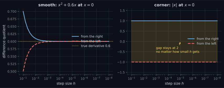
The quotient does not settle on one number as $h \to 0$; it settles on two, depending on the sign of $h$. That is what “the limit does not exist” looks like when you compute it.

See it move

Drag the gap $h$ towards zero and watch the secant line become the tangent. Switch the function with the second knob: on the smooth ones the two secants converge; on the corner they converge to different lines, which is non-differentiability made visible.

sketch A secant line becomes a tangent — unless there is a corner p5.js Pause Restart

The blue line is the secant through x and x+h. Drag h towards zero and it rotates onto the tangent. Switch to the absolute value or ReLU and drag h through zero: the left and right secants settle on different slopes, so no tangent exists.

Set the function to |x|, put $x$ at $0$, then drag $h$ all the way down. On the smooth functions the two slope readouts converge. On the corner they stay stubbornly at $-1$ and $+1$ no matter how small $h$ gets — and that is the limit failing to exist, watched rather than asserted.

On real data

figure Continuous and differentiable, continuous only, neither matplotlib

The middle panel is the one to remember: the pen never lifts, so it is continuous, but the corner means there is no single tangent. ReLU has exactly this shape.

figure The difference quotient as h shrinks matplotlib

Left: both sides settle on the same number, so the derivative exists. Right: they settle on two numbers, which is what a non-existent limit looks like numerically.

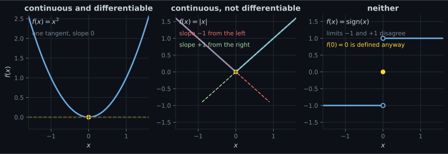
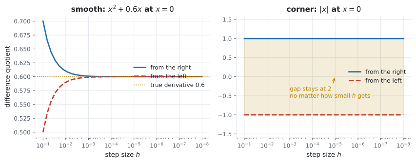
Reading the plot

In the right-hand panel of the second figure, the gap between the two curves does not narrow. It is constant at $2$ all the way down to $h = 10^{-8}$, and it would stay $2$ if you continued. That matters because it distinguishes a genuine non-differentiability from a numerical artefact: a real derivative shows the two branches converging as $h$ shrinks, until floating-point noise takes over somewhere around $h \approx 10^{-8}$ and they start to diverge again. Noise-driven divergence gets worse as $h$ shrinks; a corner’s gap is flat.

That distinction is how §5.5’s gradient-checking recipe knows the difference between a bug and a kink.

Pitfalls

The codomain is a choice, the image is not

$f(x) = x^2$ is not surjective as a map $\mathbb{R}\to\mathbb{R}$, but it is surjective as a map $\mathbb{R}\to[0,\infty)$. Same rule, different declared codomain, different answer. So “is $f$ surjective?” is not a question about the rule alone — you have to be told the codomain.

Continuous does not mean smooth

“Smooth” usually means differentiable, often infinitely so. Continuous is weaker. Every piecewise-linear activation function in deep learning lives in the gap: continuous, not differentiable everywhere.

A limit says nothing about the value at the point

$\lim_{x\to a} f(x)$ can exist while $f(a)$ is undefined, or defined and different. All three continuity conditions have to be checked separately, and the derivative definition exploits exactly this: the difference quotient is undefined at $h = 0$ and has a limit there anyway.

One-sided limits are not a technicality

They are where every counterexample lives. When a limit “does not exist”, the reason is almost always that the two sides disagree. Checking both sides is the first thing to do, not the last.

Compare

property	means	matrix version (§2.7)	why you care
injective	no two inputs collide	$\ker(\mathbf{A}) = \{\mathbf{0}\}$; columns independent	at most one solution to $\mathbf{A}\mathbf{x}=\mathbf{b}$
surjective	every target is reached	$\operatorname{Im}(\mathbf{A}) = \mathbb{R}^m$; full row rank	at least one solution, for every $\mathbf{b}$
bijective	both	square and invertible; $\det \neq 0$	exactly one solution, always
continuous	no jumps	—	the function is well-behaved enough to optimise
differentiable	one tangent	—	gradient descent has something to follow

pch.quizTag Check yourself

1. A function has an inverse exactly when it is which of these?

   A Injective B Surjective C Bijective D Continuous
   pch.quizShowAnswer

   C — Bijective — Injective alone leaves some targets with no preimage; surjective alone leaves some targets with several. Only both together give a well-defined inverse — which is the condition Chapter 2 turns into matrix invertibility.

2. ReLU is continuous everywhere but not differentiable at zero. Why not?

   A It jumps at zero B It is undefined at zero C The slope approaching from the left is zero and from the right is one, so the two-sided limit does not exist D Its derivative is infinite at zero
   pch.quizShowAnswer

   C — The slope approaching from the left is zero and from the right is one, so the two-sided limit does not exist — There is no jump, so it is continuous. But the difference quotient tends to zero from one side and one from the other, and a derivative is a two-sided limit. Frameworks return zero there by convention.

3. Sine of x divided by x is undefined at zero, yet its limit there is one. What does that make the discontinuity?

   A Removable — defining the value at zero to be one makes it continuous B A jump discontinuity that cannot be fixed C An infinite discontinuity D Not a discontinuity at all
   pch.quizShowAnswer

   A — Removable — defining the value at zero to be one makes it continuous — Both sides approach the same value, so filling in that value repairs it. Contrast the sign function, where the two sides approach different values and no choice of value at zero can help.

4. For a linear mapping, checking injectivity reduces to what?

   A Comparing every pair of inputs B Checking that only the zero vector maps to zero C Checking the codomain equals the image D Checking the function is continuous
   pch.quizShowAnswer

   B — Checking that only the zero vector maps to zero — Linearity turns the all-pairs condition into a single homogeneous system: the kernel is trivial. That collapse is what makes linear algebra computationally tractable.

🧪 Try It Yourself

Exercise 1 – The image is smaller than the codomain

pch.exerciseTag pch.exerciseTitle

Exercise 2 – Injectivity fails when outputs collide

pch.exerciseTag pch.exerciseTitle

Exercise 3 – One-sided limits of the sign function

pch.exerciseTag pch.exerciseTitle

Exercise 4 – The difference quotient of ReLU at zero

pch.exerciseTag pch.exerciseTitle

Exercise 5 – Convergence versus a constant gap

pch.exerciseTag pch.exerciseTitle

From the book

Mathematics for Machine Learning introduces these ideas where it needs them rather than in a preliminary chapter. Definition 2.16 gives injective, surjective and bijective for mappings, and §2.7 immediately applies them: a linear mapping is injective iff $\ker(\Phi) = \{\mathbf{0}\}$ (a Remark in §2.7.3, just after Figure 2.12), and an isomorphism is defined as a linear, bijective mapping, with Theorem 2.17 adding that two finite-dimensional spaces are isomorphic exactly when their dimensions agree. $\operatorname{Im}(\Phi)$ and $\ker(\Phi)$ are defined in Definition 2.23, with the rank-nullity theorem (Theorem 2.24) relating their dimensions. §5.1 defines the derivative as the limit of the difference quotient (Equation 5.3) and notes that a function must be continuous to be differentiable. The notation $\forall$, $\exists$, $\circ$, $\operatorname{Im}$ and $\ker$ is from the Table of Symbols on page 6.

Recall card

• A function is three things — domain, codomain, and a rule giving exactly one output per input.
• The image can be smaller than the codomain, and that gap is exactly what “no solution to Ax = b” means.
• Injective — different inputs never collide, so at most one solution exists.
• Surjective — every element of the codomain is reached, so at least one solution exists for every target.
• An inverse exists exactly when the function is bijective — the sentence Chapter 2 turns into matrix invertibility.
• For a linear map, injective means the kernel is trivial, which turns an all-pairs check into one homogeneous system.
• A limit requires both sides to agree and says nothing about the value at the point.
• Continuity needs all three conditions: defined, limit exists, and the two are equal.
• Differentiable implies continuous, never the reverse — ReLU is continuous everywhere and non-differentiable at zero, where frameworks return zero by convention.
• A corner’s one-sided gap stays constant as h shrinks, while floating-point noise grows — which is how gradient checking distinguishes a kink from a bug.

Next: the derivative rules themselves, derived rather than listed — Single-Variable Calculus Refresher.