Problem Setting

Chapter 9 fitted a function to labelled data. Chapter 10 has no labels at all — only $\mathbf{x}$, and a request: “find projections $\tilde{\mathbf{x}}_n$ of data points $\mathbf{x}_n$ that are as similar to the original data points as possible, but which have a significantly lower intrinsic dimensionality.”

This page is §10.1: three equations, one worked example, and a phrase in Equation 10.1’s preamble that decides whether any of it works.

What you’ll learn

• Equations 10.1–10.3: the data covariance matrix, the code $\mathbf{z} = \mathbf{B}^\top\mathbf{x}$, and the projection matrix $\mathbf{B}$.
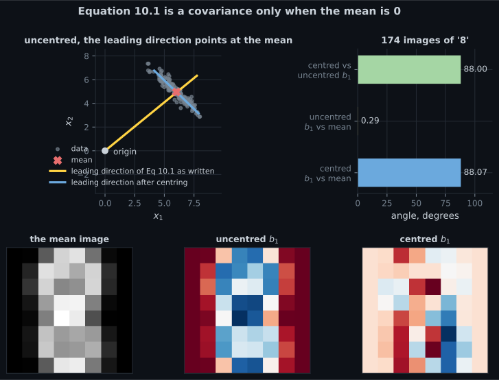
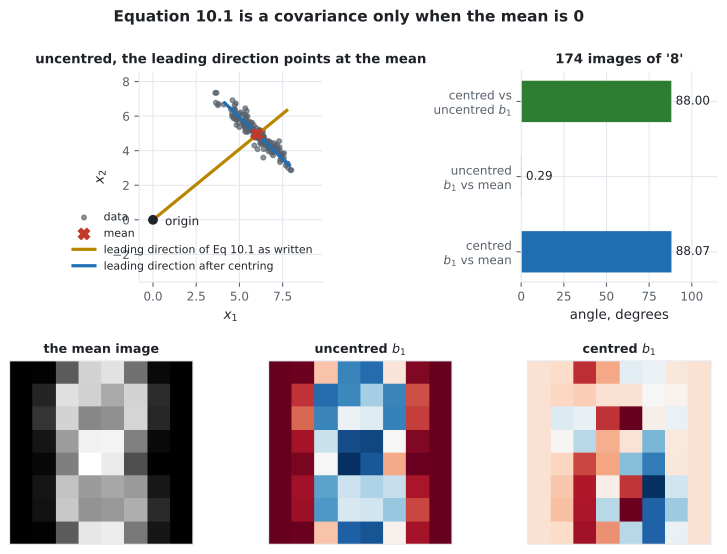
• The four words “with mean $\mathbf{0}$” attached to Equation 10.1 — and what breaks without them. Measured on $174$ images of the digit “8”: the leading direction moves $87.9996^\circ$, landing $0.2851^\circ$ from the mean image, which says nothing about how the digits differ.
• Why $\mathbf{B}^\top\mathbf{B}$ and $\mathbf{B}\mathbf{B}^\top$ are different objects. The first is $\mathbf{I}_M$ exactly; the second is $D\times D$ with $\mathrm{tr} = M$ — §10.3 will call it “the best rank-$M$ approximation of the identity”.
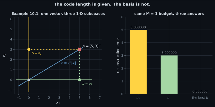
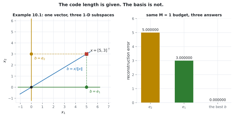
• Example 10.1, run three ways: the same $M = 1$ budget gives reconstruction errors $5.000000$, $3.000000$ and $0.000000$. Choosing $\mathbf{b}$ is the entire rest of the chapter.
• The book’s own notation warning: data points are the columns of $\mathbf{X}$ here, not the rows. Every matrix shape in Chapter 10 depends on it.
• What “overcomplete” measures out to: rank $52$ of $64$, $12$ pixels with exactly zero variance, and $57$ of $1326$ pixel pairs correlated above $0.5$.

Intuition: a bottleneck you choose the shape of

Compression is a promise about what you are allowed to forget. Figure 10.2 draws it as a funnel: $\mathbf{x} \in \mathbb{R}^D$ goes in, a code $\mathbf{z} \in \mathbb{R}^M$ comes out the narrow part, and a reconstruction $\tilde{\mathbf{x}} \in \mathbb{R}^D$ comes out the far side. The reconstruction has $D$ numbers in it again — but only $M$ of them are free.

Two decisions live in that picture and they are not the same decision:

How narrow is the neck? That is $M$, and it is yours to pick. It fixes the storage bill and nothing else.

Which directions survive it? That is $\mathbf{B}$, and §10.1 does not answer it. It only says the columns are orthonormal. Example 10.1 below shows two bases with the identical $M = 1$ budget producing errors of $5$ and $3$ on the same vector — and a third reaching $0$. §10.2 and §10.3 are two derivations of the same answer to this second question.

diagram Figure 10.2, and which arrow each section is about mermaid

  flowchart LR
  X["x in R^D
original"] -->|"encoder B'"| Z["z in R^M
code"]
  Z -->|"decoder B"| XT["x~ = BB'x in R^D
reconstructed"]
  X -.->|"the error we pay"| XT
  Z --> S1["10.1 fixes M
and says B'B = I"]
  XT --> S2["10.2 maximise the variance kept
10.3 minimise the error paid
same B"]

§10.1 The three equations

The dataset is i.i.d., $\mathcal{X} = \{\mathbf{x}_1, \ldots, \mathbf{x}_N\}$ with $\mathbf{x}_n \in \mathbb{R}^D$, with mean $\mathbf{0}$, and it “possesses the data covariance matrix”

$$\mathbf{S} = \frac{1}{N}\sum_{n=1}^{N} \mathbf{x}_n\mathbf{x}_n^\top \qquad \text{(10.1)}$$

There is assumed to exist a low-dimensional compressed representation (code)

$$\mathbf{z}_n = \mathbf{B}^\top\mathbf{x}_n \in \mathbb{R}^M \qquad \text{(10.2)}$$

with the projection matrix

$$\mathbf{B} := [\mathbf{b}_1, \ldots, \mathbf{b}_M] \in \mathbb{R}^{D\times M} \qquad \text{(10.3)}$$

whose columns are orthonormal: $\mathbf{b}_i^\top\mathbf{b}_j = 0$ for $i \neq j$ and $\mathbf{b}_i^\top\mathbf{b}_i = 1$. The projected data are $\tilde{\mathbf{x}} = \mathbf{B}\mathbf{B}^\top\mathbf{x} \in \mathbb{R}^D$, living in a subspace $U \subseteq \mathbb{R}^D$ with $\dim(U) = M < D$.

Read the shapes, then read the book’s own warning

Throughout this chapter, we do not follow the convention of collecting data as the rows of the data matrix, but we define them to be the columns of $\mathbf{X}$.

So $\mathbf{X} \in \mathbb{R}^{D\times N}$, and $\mathbf{S} = \frac{1}{N}\mathbf{X}\mathbf{X}^\top$ is $D\times D$. Almost every other textbook, and every scikit-learn array you will meet, is the transpose of this. The book gives its reason plainly: “the algebra operations work out smoothly without the need to either transpose the matrix or to redefine vectors as row vectors.”

It is worth the five seconds to check: for the digit-”8” images used below, sklearn hands you a $174\times 64$ array and the book wants the $64\times 174$ one. Getting this backwards produces a $174\times174$ “covariance matrix” that will happily decompose and mean nothing.

symbol	shape	what it is
$\mathbf{x}_n$	$D\times 1$	one data point
$\mathbf{X}$	$D\times N$	all of them, as columns
$\mathbf{S}$	$D\times D$	Equation 10.1
$\mathbf{B}$	$D\times M$	Equation 10.3, orthonormal columns
$\mathbf{z}_n$	$M\times 1$	the code, Equation 10.2
$\mathbf{B}^\top\mathbf{B}$	$M\times M$	exactly $\mathbf{I}_M$
$\mathbf{B}\mathbf{B}^\top$	$D\times D$	a projection, rank $M$

The four words that carry the weight

Equation 10.1 is introduced as “the data covariance matrix”. It is one only because of the clause before it: “with mean $\mathbf{0}$”. Written out, $\frac{1}{N}\sum \mathbf{x}_n\mathbf{x}_n^\top$ is the matrix of second moments, and the covariance is

$$\mathrm{Cov}[\mathcal{X}] = \frac{1}{N}\sum_{n=1}^{N}\mathbf{x}_n\mathbf{x}_n^\top - \boldsymbol\mu\boldsymbol\mu^\top$$

The two agree exactly when $\boldsymbol\mu = \mathbf{0}$ and not otherwise. §10.6 will list centring as “Step 1” and call it “not strictly necessary but reduces the risk of numerical problems” — which understates it. Measured on the running dataset:

quantity	value
$\lVert\boldsymbol\mu\rVert$ of the raw images	$57.264578$
$\max\lvert\mathbf{S}_{\text{raw}} - \mathbf{S}_{\text{centred}}\rvert$	$196.805423$
and that gap is $\boldsymbol\mu\boldsymbol\mu^\top$, to	$5.7\times10^{-14}$
$\mathrm{tr}(\mathbf{S}_{\text{centred}})$ — the total variance	$741.158872$
$\mathrm{tr}(\mathbf{S}_{\text{raw}})$	$4020.390805$, a factor of $\mathbf{5.4245}$

The trace is what §10.2 is about to start maximising, so inflating it by $5.4$ is not a rounding concern. Where it actually lands:

angle between	degrees
centred $\mathbf{b}_1$ and the mean image	$88.0699$
uncentred $\mathbf{b}_1$ and the mean image	$\mathbf{0.2851}$
centred $\mathbf{b}_1$ and uncentred $\mathbf{b}_1$	$87.9996$

figure Equation 10.1 is a covariance only when the mean is zero matplotlib

Skip the centring and the leading direction rotates 87.9996 degrees, to within 0.2851 degrees of the mean image — a direction along which every data point has nearly the same coordinate, and which therefore carries almost no information about how the digits differ from each other. The bottom row is the same statement as pictures.

Why the uncentred answer is degenerate, not merely different

It is not that the uncentred direction is a worse choice among reasonable ones. It is that $\frac{1}{N}\sum\mathbf{x}_n\mathbf{x}_n^\top$ measures distance from the origin, and the origin is an arbitrary point that has nothing to do with the data. When $\lVert\boldsymbol\mu\rVert$ is large compared with the spread — here $57.26$ against a total standard deviation of $\sqrt{741.16} = 27.22$ — the sum is dominated by $N\boldsymbol\mu\boldsymbol\mu^\top$, a rank-one matrix whose only eigenvector with a nonzero eigenvalue is $\boldsymbol\mu$ itself.

So the first “principal component” comes back as the mean, and the first coordinate $z_{1n}$ is approximately the same number for every $n$. You have spent your entire $M = 1$ budget storing a constant.

Example 10.1, and the question §10.1 does not answer

The book’s example is deliberately plain: in $\mathbb{R}^2$ with the canonical basis, $[5, 3]^\top = 5\mathbf{e}_1 + 3\mathbf{e}_2$, while any vector of the form $[0, z]^\top$ needs only the single coordinate $z$ with respect to $\mathbf{e}_2$. The set of such vectors is a subspace with $\dim(U) = 1$, because $U = \mathrm{span}[\mathbf{e}_2]$.

Run it as a compression problem instead, on the vector $[5,3]^\top$ itself, with $M = 1$ throughout:

basis $\mathbf{b}$	code $\mathbf{z}$	$\tilde{\mathbf{x}}$	$\lVert\mathbf{x} - \tilde{\mathbf{x}}\rVert$
$\mathbf{e}_2$	$[3]$	$[0, 3]^\top$	$5.000000$
$\mathbf{e}_1$	$[5]$	$[5, 0]^\top$	$3.000000$
$\mathbf{x}/\lVert\mathbf{x}\rVert$	$[5.830952]$	$[5, 3]^\top$	$\mathbf{0.000000}$

figure One code length, three bases, three answers matplotlib

Every row spends exactly one number. The book's Section 10.1 fixes M and requires orthonormal columns, and stops there — nothing said so far prefers any of these three. Sections 10.2 and 10.3 are two different derivations of the same preference.

One data point is a special case, and it is worth knowing why

With a single vector, the perfect basis is the vector itself, and a code of length $1$ is lossless. That is $\mathbf{S} = \frac{1}{1}\mathbf{x}\mathbf{x}^\top$, a rank-one matrix: one nonzero eigenvalue, $\lVert\mathbf{x}\rVert^2 = 34$, with eigenvector $\mathbf{x}/\lVert\mathbf{x}\rVert$.

The whole difficulty of PCA arrives with the second data point, when one direction has to serve two vectors that disagree about which direction is best.

The bottleneck, on a real image

The book’s running example is MNIST: $60{,}000$ handwritten digits at $28\times28$ pixels, so $\mathbf{x} \in \mathbb{R}^{784}$. The pages here use the $8\times8$ version of the same corpus that ships inside scikit-learn, which needs no download and reproduces to the digit — $D = 64$, and $N = 174$ images of the digit “8”. Everything on this page scales; only the numbers change.

figure The reconstruction has 64 numbers in it and M degrees of freedom matplotlib

The top row is Figure 10.2 run end to end. Each reconstruction is a full 64-pixel image, but the matrix of all 174 of them has rank exactly M — measured at 1, 2, 5, 10 and 20. The bottom row is what was thrown away: the residual visibly drains as M grows, and the error norm falls 25.92, 23.99, 20.06, 15.36, 9.35.

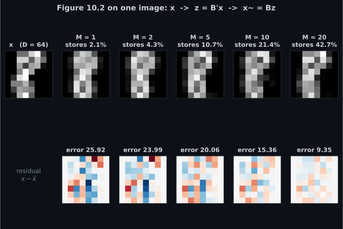
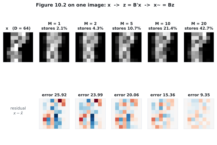
The storage arithmetic is worth doing once, because it is the only reason to compress at all. Keeping the codes and the basis costs $NM + DM = M(N+D)$ numbers against $ND$ raw:

$M$	rank of $\tilde{\mathbf{X}}$	numbers stored	share of $11{,}136$
$1$	$1$	$238$	$2.1\%$
$2$	$2$	$476$	$4.3\%$
$5$	$5$	$1190$	$10.7\%$
$10$	$10$	$2380$	$21.4\%$
$20$	$20$	$4760$	$42.7\%$

The basis is a fixed cost, and with few data points it dominates

$M(N+D) < ND$ fails once $M \geq \frac{ND}{N+D}$. Here that is $11136/238 = 46.79$, so $M = 47$ or more stores more numbers than the raw data — even though $M = 47$ is still a genuine dimensionality reduction from $D = 64$.

With $N = 60{,}000$ MNIST images the basis is negligible and the ratio is essentially $M/D$. With $N$ comparable to $D$ it is not, and that asymmetry is exactly the regime §10.5 is written for.

Two matrices that are easy to confuse

$\mathbf{B}^\top\mathbf{B}$ and $\mathbf{B}\mathbf{B}^\top$ are built from the same $D\times M$ matrix and are nothing alike.

$$\mathbf{B}^\top\mathbf{B} = \mathbf{I}_M \in \mathbb{R}^{M\times M}, \qquad \mathbf{B}\mathbf{B}^\top = \sum_{m=1}^{M}\mathbf{b}_m\mathbf{b}_m^\top \in \mathbb{R}^{D\times D}$$

The first is the orthonormality assumption restated. The second is the projection onto $\mathrm{span}[\mathbf{b}_1,\ldots,\mathbf{b}_M]$ — §10.3 arrives at it as Equation 10.39 and notes it is “the best rank-$M$ approximation of the identity matrix”. Measured, using the same tests page 909 ran on the linear-regression hat matrix:

$M$	$\lvert\mathbf{B}^\top\mathbf{B} - \mathbf{I}\rvert$	$\lvert P^2 - P\rvert$	$\lvert P - P^\top\rvert$	$\mathrm{tr}(P)$
$1$	$4.4\times10^{-16}$	$6.9\times10^{-17}$	$0.0$	$1.000000$
$2$	$3.3\times10^{-16}$	$8.3\times10^{-17}$	$0.0$	$2.000000$
$5$	$6.7\times10^{-16}$	$2.2\times10^{-16}$	$0.0$	$5.000000$
$10$	$1.3\times10^{-15}$	$4.2\times10^{-16}$	$0.0$	$10.000000$

The trace of a projection is its rank, which is the same fact page 909 used to explain Equation 9.22’s $(N-K)/N$ bias. Chapter 10 will use it again in Equation 10.43b.

What “overcomplete” actually measures

The chapter’s opening claim is that high-dimensional data “is often overcomplete, i.e., many dimensions are redundant and can be explained by a combination of other dimensions”, and that dimensions “are often correlated so that the data possesses an intrinsic lower-dimensional structure.” On the digit-”8” images:

claim	measurement
dimensions are redundant	the centred $64\times174$ matrix has rank $\mathbf{52}$, not $64$
some carry nothing at all	$\mathbf{12}$ pixels have exactly zero variance; $19$ have variance below $1$
dimensions are correlated	mean $\lvert\text{corr}\rvert$ between live pixels $= 0.152872$
strongly, in places	$\mathbf{57}$ of $1326$ pixel pairs exceed $\lvert\text{corr}\rvert = 0.5$

Twelve dead pixels is a free dimensionality reduction that needs no eigendecomposition: they are the image border, always black in every “8”. The other $12$ lost ranks are the interesting part — no single pixel is redundant, but the $52$ live directions span everything.

pch.quizTag Is the setup clear?

1. Equation 10.1 defines S as the average of x x-transpose. When is that the data covariance matrix?

   A Always — it is the definition of covariance B Only when the data has mean zero; otherwise it exceeds the covariance by mu mu-transpose C Only when the data is Gaussian D Only when N is larger than D
   pch.quizShowAnswer

   B — Only when the data has mean zero; otherwise it exceeds the covariance by mu mu-transpose — Measured on 174 images of the digit 8: the gap between the raw second-moment matrix and the true covariance matches mu mu-transpose to 5.7e-14, the trace is inflated by a factor of 5.4245, and the leading direction rotates 87.9996 degrees onto the mean image itself — 0.2851 degrees from it.

2. B is D-by-M with orthonormal columns. What is B-transpose times B, and what is B times B-transpose?

   A Both are the identity B B-transpose B is the M-by-M identity; B B-transpose is D-by-D with rank M and trace M C B-transpose B is D-by-D; B B-transpose is M-by-M D Neither is symmetric
   pch.quizShowAnswer

   B — B-transpose B is the M-by-M identity; B B-transpose is D-by-D with rank M and trace M — Measured at M = 1, 2, 5 and 10: B-transpose B matches the identity to 1.3e-15 at worst, while B B-transpose is exactly symmetric, idempotent to 4.2e-16, and has trace exactly M. The trace of a projection is its rank — the same fact page 909 used on the regression hat matrix.

3. Section 10.1 fixes M and requires orthonormal columns. What does it NOT do?

   A It does not say what D is B It does not choose the basis — nothing in Section 10.1 prefers one orthonormal B over another C It does not allow the data to be centred D It does not define the reconstruction
   pch.quizShowAnswer

   B — It does not choose the basis — nothing in Section 10.1 prefers one orthonormal B over another — Example 10.1 run as a compression problem: the vector [5, 3] with M = 1 gives reconstruction errors 5.000000 with b = e2, 3.000000 with b = e1, and 0.000000 with b along x itself. Same budget, same orthonormality, three answers. Sections 10.2 and 10.3 are two derivations of the same choice.

4. For the 174 digit-8 images with D = 64, at what M does storing codes plus basis stop saving anything?

   A M = 64, when the code is as long as the data B M = 47, because the basis costs D*M numbers on top of the N*M codes C M = 32, half of D D It always saves, for any M less than D
   pch.quizShowAnswer

   B — M = 47, because the basis costs D*M numbers on top of the N*M codes — M(N + D) < N*D fails at M >= 11136/238 = 46.79. The basis is a fixed cost paid once, so it only disappears when N is large — with 60,000 MNIST images it is negligible and the ratio is essentially M/D. When N is comparable to D it is not, which is the regime Section 10.5 addresses.

Exercises

Exercise 1 – Equation 10.1 is a covariance only if you centre

pch.exerciseTag pch.exerciseTitle

Exercise 2 – Where the uncentred direction actually points

pch.exerciseTag pch.exerciseTitle

Exercise 3 – Two matrices, two shapes, one projection

pch.exerciseTag pch.exerciseTitle

Exercise 4 – Example 10.1 as a compression problem

pch.exerciseTag pch.exerciseTitle

Exercise 5 – When does compressing stop saving anything?

pch.exerciseTag pch.exerciseTitle

Recall card

• Chapter 10 has no labels. The data is just x, and the request is a projection of it that keeps most of what the original said while needing far fewer numbers.
• Equation 10.1’s S is the data covariance matrix only because the data is assumed to have mean zero. Applied to raw data it is the second-moment matrix, larger by the outer product of the mean with itself.
• Measured on 174 images of the digit eight, skipping the centring moves the leading direction by 87.9996 degrees, to within 0.2851 degrees of the mean image — a direction on which every point has nearly the same coordinate.
• It also inflates the total variance by a factor of 5.4245, and the total variance is exactly what Section 10.2 is about to maximise.
• The code is z = B-transpose x and the reconstruction is x-tilde = B B-transpose x. B is D by M with orthonormal columns.
• B-transpose B is the M by M identity; B B-transpose is D by D with rank M. They are built from the same matrix and are not the same object.
• The trace of B B-transpose is exactly M, measured at M equal to 1, 2, 5 and 10. The trace of a projection is its rank, which is the same fact page 909 used on the regression hat matrix.
• Section 10.1 fixes the code length and requires orthonormality, and chooses nothing else. Example 10.1’s vector with M equal to one gives errors of 5, 3 and 0 under three different orthonormal bases.
• Chapter 10 stores data points as the columns of X, not the rows, so X is D by N and every shape in the chapter follows from that.
• Storage costs M times N plus D, against N times D raw. With 174 images and 64 pixels, a code of length 47 already saves nothing, because the basis is a fixed cost paid once.
• Overcomplete, measured: the 64 by 174 centred matrix has rank 52, twelve pixels have exactly zero variance, and 57 of 1326 pixel pairs are correlated above one half.

Next: The Maximum Variance Perspective — the first of two derivations that answer the question §10.1 leaves open, by asking which direction keeps the most variance.