Serving Models with TensorFlow Serving

A trained model in a notebook is reachable by exactly one thing: that notebook. Serving is the step that makes it reachable by anything else, and the failure mode it introduces is unlike anything in training — the model keeps working, keeps returning plausible numbers, and is wrong.

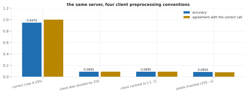
Here is that failure, measured. The same served model, four clients that preprocess their input slightly differently:

Client preprocessing	Accuracy	Agreement	Mean confidence
Correct (raw 0–255)	0.9470	1.0000	0.9416
Also divided by 255	0.0895	0.0900	0.1431
Centred to [−1, 1]	0.0895	0.0900	0.1452
Pixels inverted	0.0850	0.0795	0.8061

Every one of those calls succeeded. No exception, no warning, no shape error. The last row is the worst: 8.5% accurate while reporting 0.81 average confidence. A production server has no way to notice this without labels, which it does not have.

What “export” actually writes

Exporting for serving

model.export("served/1")            # note the version number in the path

File	Size
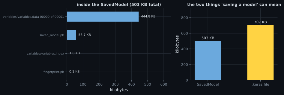
`variables/variables.data-00000-of-00001`	444.8 KB
`saved_model.pb`	56.7 KB
`variables/variables.index`	1.0 KB
`fingerprint.pb`	0.1 KB
Total	502.6 KB
The same model as `.keras`	707.1 KB

Two things in that listing matter.

The graph is separate from the weights. saved_model.pb is the computation — a language-independent protocol buffer that a C++ server can execute without Python. The weights sit beside it. That separation is what makes serving possible at all; a .keras file is a Python artefact that needs Keras to reconstitute.

The path ends in a version number. TF Serving watches the parent directory, and when served/2 appears it loads it, waits for in-flight requests to served/1 to finish, and then drops the old one. Version numbers in the directory layout are the entire deployment mechanism.

Left: horizontal bars of the files inside the SavedModel directory, dominated by the variables data file at 444.8 KB with saved_model.pb at 56.7 KB. Right: two bars comparing the SavedModel total of 502.6 KB against the .keras file at 707.1 KB. — The SavedModel is smaller than the .keras file despite containing the same weights, because it stores the executable graph rather than the configuration needed to rebuild the model in Python for further training. It is a deployment artefact: everything required to run the forward pass, and nothing required to continue training.

The signature is the API contract

text

signatures: ['serve', 'serving_default']
  input   image        shape [-1, 28, 28, 1]  float32
  output  output_0     shape [-1, 10]         float32

This is what a client codes against, and it is worth reading carefully.

The −1 is the batch dimension: the signature accepts any number of images per request. That single detail is what makes server-side batching possible.

The name image is what a REST or gRPC caller uses as a key. Rename that input layer and every client breaks — the signature is a public interface, and it should be treated with the same care as any other API.

What a REST client sends

{"instances": [[[0.0], [0.0], ...]]}          # shape must match [-1, 28, 28, 1]

Nothing in that payload says what units the pixels are in. The shape is checked; the meaning is not.

Batching is why servers are fast

Left: per-request and per-sample latency against batch size on log axes. Per-request rises from 1.352 ms at batch 1 to 12.379 ms at batch 128, while per-sample falls from 1.3521 ms to 0.0967 ms. Right: throughput rising from 740 samples per second at batch 1 to 10,340 at batch 128. — Per-sample cost falls 14.0x from batch 1 to batch 128 while per-request latency rises only 9.2x. That gap is the fixed overhead of a request — graph dispatch, tensor allocation, the call itself — being spread over more samples. It is why TF Serving has a batching scheduler that waits a few milliseconds to accumulate requests before running them together.

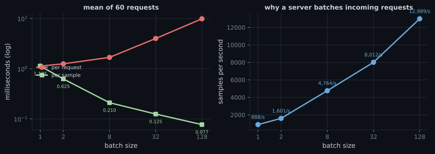
Batch	ms/request	ms/sample	Samples/s
1	1.352	1.3521	740
8	1.598	0.1997	5,007
32	4.744	0.1482	6,745
128	12.379	0.0967	10,340

The trade is explicit: batching improves throughput and worsens the latency of any individual request, because a request must wait for the batch to fill. A server tuning this sets a maximum wait time — collect requests for up to N milliseconds, then run whatever has arrived.

Note also that batch 2 was slightly faster per request than batch 1 (1.274 ms against 1.352). At these sizes the measurement is dominated by fixed overhead, and small differences between adjacent batch sizes are noise rather than signal.

Training/serving skew

figure The same server, 2,000 digits, four client conventions matplotlib

This is the deployment failure that does not announce itself. The model was trained on raw 0-255 pixels with a Rescaling layer inside it; a client that helpfully divides by 255 first sends values in [0, 0.004] after the model's own rescaling, and the network has never seen anything like them. Accuracy falls from 0.9470 to 0.0895 — worse than guessing — and the request still returns a valid probability vector.

diagram Diagram mermaid

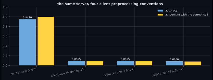
  flowchart LR
  C["client"] -->|"raw 0-255 pixels"| S["SavedModel"]
  S --> R["Rescaling(1/255) INSIDE the model"]
  R --> N["convnet"]
  N --> P["probabilities"]
  C -.->|"client divides by 255 first"| W["values in 0 to 0.004"]
  W -.->|"no error, no warning"| B["accuracy 0.0895,
confidence 0.1431"]

The defence is structural, not procedural: put the preprocessing inside the model.

Preprocessing that ships with the weights

inputs = keras.layers.Input((28, 28, 1), name="image")
x = keras.layers.Rescaling(1.0 / 255.0)(inputs)      # travels with the model
x = keras.layers.Conv2D(16, 3, activation="relu")(x)

Once the Rescaling layer is part of the exported graph, the contract is “send raw pixels” and there is nothing for a client to get wrong. Anything left outside the model has to be reproduced exactly by every caller, in every language, forever — and each one is an opportunity for the table above.

The inverted-pixels row deserves a second look: 0.8061 mean confidence at 8.5% accuracy. High confidence is not evidence of correct input. A monitoring system watching only confidence would have seen nothing wrong.

sketch The batching trade p5.js

Drag the maximum batch size and the maximum wait. The bars show how long a request spends queueing against computing, and the resulting throughput.

What to monitor instead

Since accuracy is unavailable in production, monitor the things that are:

Input distribution. Mean, standard deviation and range per feature, compared against training. The double-scaled client would have shown a mean 255× too small immediately.
Prediction distribution. If a balanced classifier suddenly returns 80% one class, something upstream changed.
Confidence distribution, but as a shape, not a threshold — the inverted-pixel row proves a high mean confidence can accompany near-random predictions.
Latency percentiles, not the mean. The mean hides the batching tail.
Version and traffic split, so a regression can be attributed to a specific deployment.

sketch The measured table, ranked p5.js

Click a column to rank every row by it. The bars are that column's values and the highest and lowest are computed from the numbers, not written in.

Pitfalls

Leaving preprocessing outside the model. 0.9470 → 0.0895 with no error raised.
Trusting confidence as a health signal. The worst variant had the second-highest confidence at 0.8061.
Renaming an input layer after clients exist. The layer name is the API key in the request payload.
Exporting without a version directory. TF Serving’s whole hot-swap mechanism keys off .../1, .../2.
Serving a .keras file. It is a Python artefact; the server needs the SavedModel graph.
Benchmarking with batch 1 and provisioning for it. Per-sample cost fell 14× by batch 128.
Reading small differences between adjacent batch sizes. Batch 2 beat batch 1 here; that is overhead noise.

Recap

model.export() writes a versioned SavedModel: an executable graph (56.7 KB) plus weights (444.8 KB), smaller than the 707.1 KB .keras file because it drops everything training-only.
The serving signature is a public API — input names and the −1 batch dimension are the contract.
Batching cut per-sample cost 14.0× from batch 1 to 128, at the price of per-request latency.
A client preprocessing differently from training dropped accuracy to 0.0895 with no error.
Inverted pixels produced 0.8061 mean confidence at 0.0850 accuracy, so confidence is not a health check.
Put preprocessing inside the model, and monitor input distributions rather than only outputs.

That is the deployment path end to end. The last page of the phase steps back and asks what this whole approach still cannot do: Limitations and the Future of Deep Learning.

pch.quizTag pch.quizDefaultTitle

A client divided its pixels by 255 before sending them to a model that already contains a Rescaling layer. Accuracy fell from 0.9470 to 0.0895. Why did nothing raise an error?

pch.quizShowAnswer

B — The request had the correct shape and dtype — only the meaning of the values was wrong, and nothing in the signature describes units — Shape and dtype are checked; semantics are not. This is why preprocessing belongs inside the exported graph.
The inverted-pixel client scored 0.0850 accuracy with 0.8061 mean confidence. What does that rule out?

pch.quizShowAnswer

B — Using confidence as a health check — a model can be confidently wrong on out-of-distribution input, so high average confidence is not evidence that the input is correct — It scored the second-highest confidence of the four variants while being the least accurate, which is exactly the case a confidence threshold would miss.
Why does the SavedModel directory path end in a version number?

pch.quizShowAnswer

B — TF Serving watches the parent directory — when a higher-numbered version appears it loads it, drains in-flight requests to the old one, and unloads it, which is the whole hot-swap mechanism — The directory layout is the deployment interface, which is why exporting without a version number breaks the server's rollout behaviour.
Per-sample cost fell from 1.3521 ms at batch 1 to 0.0967 ms at batch 128, while per-request latency rose from 1.352 ms to 12.379 ms. What is the trade?

pch.quizShowAnswer

B — Throughput against individual latency — a request must wait for its batch to fill, so servers set a maximum wait time and run whatever has accumulated — The fixed per-request overhead is spread over more samples, which is why the per-sample curve falls 14x while the per-request curve rises only 9.2x.
Why is the SavedModel (502.6 KB) smaller than the .keras file (707.1 KB) for the same model?

pch.quizShowAnswer

B — It stores an executable graph plus weights and drops everything needed only to rebuild the model in Python for further training — It is a deployment artefact: everything required to run the forward pass from C++, and nothing required to continue training.

🧪 Try It Yourself

pch.coffeeTagline

pch.coffeeCta

pch.feedbackHeading

pch.feedbackSubheading