Orthogonal Complement

Fix a subspace $U$ inside a $D$-dimensional space. Every vector in the space now splits into two parts — the part that lies in $U$, and the part that does not — and this page says three things about that split which are stronger than you might expect:

it is unique, the leftover part lives in a subspace of its own, and the two parts satisfy Pythagoras exactly.

That is the entire content of §3.6, and it is what makes “the part PCA keeps” and “the part PCA discards” well-defined objects rather than loose talk.

What you’ll learn

• The definition of the orthogonal complement $U^\perp$, and why it is a subspace rather than just a set.
• The dimension count $\dim U + \dim U^\perp = D$, and the fact that $U \cap U^\perp = \{\mathbf{0}\}$.
• Equation 3.36: the unique decomposition of any vector into a $U$-part and a $U^\perp$-part.
• Pythagoras for that split, measured over four thousand vectors in $\mathbb{R}^5$.
• Why a plane in $\mathbb{R}^3$ is described by a single normal vector, and how that generalises to hyperplanes.
• A real dataset whose orthogonal complement turns out to be spanned by exactly three coordinate axes — identified, not guessed.

Intuition: the shadow and the height

Stand a pencil on a table. Its shadow on the tabletop is the part of it that lies in the plane of the table; the height of its tip above the table is the part that does not. Two numbers-worth of shadow, one number of height, three numbers of pencil.

That accounting is exactly the dimension count. And there is only one way to do it: the shadow is determined by the pencil, and so is the height. You cannot trade a bit of shadow for a bit of height — that is the uniqueness claim.

The Pythagorean part is the one worth pausing on. The squared length of the pencil equals the squared shadow plus the squared height. Not the lengths, the squares. Which means a component that looks small contributes even less than it looks: a direction carrying $10\%$ of the length carries $1\%$ of the squared length, and squared length is what variance is.

diagram Diagram mermaid

  flowchart TD
  V["a D-dimensional space V"]
  V --> U["a subspace U, dim M"]
  U --> PERP["U-perp: every vector orthogonal to ALL of U
dim D − M"]
  PERP --> SUB["U-perp is itself a SUBSPACE
closed under sums and scaling"]
  PERP --> TRIV["U ∩ U-perp = {0}
only the zero vector is in both"]
  TRIV --> UNIQ["so x = p + q is UNIQUE
Eq 3.36"]
  UNIQ --> PYTH["and ‖x‖² = ‖p‖² + ‖q‖²
because ⟨p, q⟩ = 0"]
  PYTH --> ML["variance kept + variance lost = total
PCA, Ch 10"]
  PERP --> NORM["dim U-perp = 1 ⟹ ONE normal vector
describes the whole of U
hyperplanes, Ch 12"]

The math

Orthogonal complement

Consider a $D$-dimensional vector space $V$ and an $M$-dimensional subspace $U \subseteq V$. The orthogonal complement $U^\perp$ is the set of all vectors in $V$ that are orthogonal to every vector in $U$:

$$U^\perp = \{\, \mathbf{v} \in V : \langle \mathbf{v}, \mathbf{u}\rangle = 0 \text{ for all } \mathbf{u} \in U \,\}$$

It is a $(D-M)$-dimensional subspace of $V$, and

$$U \cap U^\perp = \{\mathbf{0}\} .$$

Three points, in order of how easy they are to overlook.

$U^\perp$ is a subspace, not merely a set. If $\mathbf{v}_1$ and $\mathbf{v}_2$ are both orthogonal to everything in $U$, then so is $\alpha\mathbf{v}_1 + \beta\mathbf{v}_2$, by bilinearity: $\langle \alpha\mathbf{v}_1 + \beta\mathbf{v}_2, \mathbf{u}\rangle = \alpha\cdot 0 + \beta\cdot 0 = 0$. So $U^\perp$ has a basis, a dimension, and everything else Chapter 2 gives a subspace.

The intersection is trivial. If $\mathbf{v}$ is in both, it is orthogonal to itself, so $\langle\mathbf{v},\mathbf{v}\rangle = 0$, so $\mathbf{v} = \mathbf{0}$ by positive definiteness. Note which axiom did the work — this is one of the places where the positive-definiteness requirement on the inner product earns its keep.

“Orthogonal to every vector in $U$” only needs checking on a basis. By bilinearity, being orthogonal to $\mathbf{b}_1, \dots, \mathbf{b}_M$ is enough to be orthogonal to every combination of them. That turns an infinite condition into $M$ equations, which is what makes $U^\perp$ computable at all: it is the null space of the matrix whose rows are a basis of $U$.

The unique decomposition

Equation 3.36

Let $(\mathbf{b}_1,\dots,\mathbf{b}_M)$ be a basis of $U$ and $(\mathbf{b}_1^\perp,\dots,\mathbf{b}_{D-M}^\perp)$ a basis of $U^\perp$. Then any $\mathbf{x} \in V$ can be written uniquely as

$$\mathbf{x} = \sum_{m=1}^{M} \lambda_m \mathbf{b}_m + \sum_{j=1}^{D-M} \psi_j \mathbf{b}_j^\perp$$

Together the two bases form a basis of $V$, since their dimensions add to $D$ and they share nothing but the origin.

Write $\mathbf{p}$ for the first sum and $\mathbf{q}$ for the second. Then $\mathbf{p} \in U$, $\mathbf{q} \in U^\perp$, and $\langle\mathbf{p},\mathbf{q}\rangle = 0$ — which gives Pythagoras with no further work:

$$\lVert\mathbf{x}\rVert^2 = \langle \mathbf{p}+\mathbf{q}, \mathbf{p}+\mathbf{q}\rangle = \lVert\mathbf{p}\rVert^2 + 2\underbrace{\langle\mathbf{p},\mathbf{q}\rangle}_{=\,0} + \lVert\mathbf{q}\rVert^2 = \lVert\mathbf{p}\rVert^2 + \lVert\mathbf{q}\rVert^2$$

The cross term vanishing is the whole proof. Everything Chapter 10 says about “variance explained” rests on this line and on nothing else.

Normal vectors and hyperplanes

The special case $\dim U^\perp = 1$ is the one you meet most often. A plane through the origin in $\mathbb{R}^3$ has $M = 2$, so its complement is one-dimensional: a single direction $\mathbf{w}$, the normal vector, describes the entire plane, because

$$U = \{\, \mathbf{x} \in \mathbb{R}^3 : \langle \mathbf{w}, \mathbf{x}\rangle = 0 \,\} .$$

Two numbers’ worth of plane, described by one vector — that is the trade a codimension-one subspace offers, and it scales: a hyperplane in $\mathbb{R}^D$ has dimension $D-1$ and is still described by one normal vector. Chapter 12 builds the support vector machine on precisely this, and the distance from a point to the plane has the closed form

$$d(\mathbf{x}, U) = \frac{\lvert \langle \mathbf{w}, \mathbf{x}\rangle \rvert}{\lVert\mathbf{w}\rVert},$$

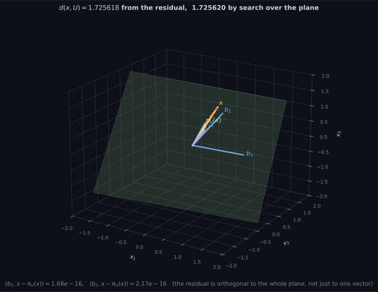
which the figures below check against a brute-force search.

From the book

Section 3.6. The orthogonal complement is defined there with the dimension count $D - M$, the trivial intersection $U \cap U^\perp = \{\mathbf{0}\}$, and the unique decomposition of Equation 3.36. Figure 3.7 draws a three-dimensional example with the normal vector of a plane. The section notes that this is what a plane is described by, and that the same construction underlies the separating hyperplane of Section 12.1.

Worked example by hand

Take the plane $U \subset \mathbb{R}^3$ spanned by

$$\mathbf{b}_1 = (1,\ 0.6,\ -0.3)^\top, \qquad \mathbf{b}_2 = (0.2,\ 1,\ 0.7)^\top$$

and the vector $\mathbf{x} = (0.9,\ -0.4,\ 1.6)^\top$.

Step 1 — find $U^\perp$. It is one-dimensional, and the cross product gives a vector orthogonal to both:

$$\mathbf{b}_1 \times \mathbf{b}_2 = \begin{bmatrix} 0.6(0.7) - (-0.3)(1) \\ (-0.3)(0.2) - 1(0.7) \\ 1(1) - 0.6(0.2) \end{bmatrix} = \begin{bmatrix} 0.42 + 0.30 \\ -0.06 - 0.70 \\ 1 - 0.12 \end{bmatrix} = \begin{bmatrix} 0.72 \\ -0.76 \\ 0.88 \end{bmatrix}$$

Its length is $\sqrt{0.5184 + 0.5776 + 0.7744} = \sqrt{1.8704} \approx 1.367626$, so the unit normal is

$$\mathbf{w} = (0.526460,\ -0.555708,\ 0.643451)^\top .$$

Step 2 — the $U^\perp$ part of $\mathbf{x}$. It is the projection onto the normal direction:

$$\langle\mathbf{w},\mathbf{x}\rangle = 0.526460(0.9) + (-0.555708)(-0.4) + 0.643451(1.6) = 1.725618$$ $$\mathbf{q} = \langle\mathbf{w},\mathbf{x}\rangle\,\mathbf{w} = (0.908469,\ -0.958939,\ 1.110351)^\top$$

Step 3 — the $U$ part is whatever is left.

$$\mathbf{p} = \mathbf{x} - \mathbf{q} = (-0.008469,\ 0.558939,\ 0.489649)^\top$$

Step 4 — check. The right thing to test is the displacement $\mathbf{x} - \mathbf{p}$, which is $\mathbf{q}$, against a basis of $U$. Testing $\mathbf{b}_1$ against $\mathbf{p}$ instead would prove nothing, because $\mathbf{p}$ lies in $U$ and has every reason to have a nonzero inner product with a basis vector of it.

check	expected	measured
$\langle\mathbf{b}_1,\mathbf{q}\rangle$	$0$	$-4.318\times10^{-17}$
$\langle\mathbf{b}_2,\mathbf{q}\rangle$	$0$	$-4.931\times10^{-17}$
$\lVert\mathbf{p}\rVert^2 + \lVert\mathbf{q}\rVert^2$	$\lVert\mathbf{x}\rVert^2 = 0.81 + 0.16 + 2.56$	$3.53$
$d(\mathbf{x}, U)$ from the residual $\lVert\mathbf{q}\rVert$	—	$1.725618$
$d(\mathbf{x}, U)$ from $\lvert\langle\mathbf{w},\mathbf{x}\rangle\rvert / \lVert\mathbf{w}\rVert$	the same	$1.725618$

The last two rows agree exactly, and they have to: for a unit normal, $\lVert\mathbf{q}\rVert = \lvert\langle\mathbf{w},\mathbf{x}\rangle\rvert \cdot \lVert\mathbf{w}\rVert = \lvert\langle\mathbf{w},\mathbf{x}\rangle\rvert$, so dividing by $\lVert\mathbf{w}\rVert$ is doing nothing. The division matters only when you skip the normalisation step and work with an unnormalised normal vector, which is the usual case in practice.

complement_worked.py

import numpy as np
 
b1 = np.array([1.0, 0.6, -0.3])
b2 = np.array([0.2, 1.0, 0.7])
x = np.array([0.9, -0.4, 1.6])
 
# U-perp is one-dimensional; the cross product spans it.
w = np.cross(b1, b2)
print("cross product:", w, " length:", np.linalg.norm(w))
w = w / np.linalg.norm(w)
print("unit normal:  ", np.round(w, 6))
 
q = float(w @ x) * w              # the U-perp part
p = x - q                         # the U part
print("<w, x> =", round(float(w @ x), 6))
print("q (in U-perp):", np.round(q, 6))
print("p (in U):     ", np.round(p, 6))
 
print("<b1, q> =", f"{b1 @ q:.3e}", "  <b2, q> =", f"{b2 @ q:.3e}")
print("Pythagoras: |p|^2 + |q|^2 =", round(float(p @ p + q @ q), 6),
      " |x|^2 =", round(float(x @ x), 6))
print("distance from the residual:", round(float(np.linalg.norm(q)), 6))
print("distance from |<w,x>|:     ", round(abs(float(w @ x)), 6))

output

cross product: [ 0.72 -0.76  0.88]  length: 1.3676256797823008
unit normal:   [ 0.52646  -0.555708  0.643451]
<w, x> = 1.725618
q (in U-perp): [ 0.908469 -0.958939  1.110351]
p (in U):      [-0.008469  0.558939  0.489649]
<b1, q> = -4.318e-17   <b2, q> = -4.931e-17
Pythagoras: |p|^2 + |q|^2 = 3.53  |x|^2 = 3.53
distance from the residual: 1.725618
distance from |<w,x>|:      1.725618

Both orthogonality checks land below $5\times10^{-17}$ and Pythagoras is exact to the printed precision. The two routes to the distance agree exactly, which they must: for a unit normal $\lVert\mathbf{q}\rVert$ is $\lvert\langle\mathbf{w},\mathbf{x}\rangle\rvert$, so the division by $\lVert\mathbf{w}\rVert = 1$ does nothing.

See it move

The first sketch is the split in the plane, where $U$ is a line and $U^\perp$ is the perpendicular line. Drag either the vector or the subspace.

sketch Every vector splits, and only one way p5.js Pause Restart

Drag the white vector x, or drag the amber handle to rotate the subspace U. The green arrow is the part of x inside U and the violet arrow is the part in U-perp. The bar chart underneath is Pythagoras: the two squared parts always fill the bar for the squared whole exactly.

The second sketch is the codimension-one case, where a single normal vector describes the whole subspace and the distance formula falls out.

sketch One normal vector describes a whole hyperplane p5.js Pause Restart

Drag the normal w and drag the point x. The line is every vector whose inner product with w is zero — the whole subspace, specified by one vector. The readout compares the closed-form distance against a brute-force scan along the line, and the two agree to the printed precision.

From scratch

complement_from_scratch.py

import numpy as np
 
def complement_basis(U_cols):
    """An orthonormal basis of the orthogonal complement of the column span.
 
    The complement is the null space of the matrix whose ROWS are a basis of U,
    and an SVD reads that off directly: the right singular vectors beyond the
    rank span it.
    """
    A = np.asarray(U_cols, dtype=float)
    _, sv, Vt = np.linalg.svd(A.T, full_matrices=True)
    rank = int(np.sum(sv > sv.max() * len(sv) * np.finfo(float).eps))
    return Vt[rank:]
 
def split(x, U_cols):
    """Decompose x into its U part and its U-perp part."""
    Q, _ = np.linalg.qr(np.asarray(U_cols, dtype=float))
    p = Q @ (Q.T @ x)
    return p, x - p
 
# Pythagoras, measured over 4000 random vectors against a fixed subspace.
rng = np.random.default_rng(23)
n, m, samples = 5, 2, 4000
Q, _ = np.linalg.qr(rng.normal(size=(n, m)))
P = Q @ Q.T
Pc = np.eye(n) - P
 
X = rng.normal(size=(samples, n)) * rng.uniform(0.3, 3.0, size=(samples, 1))
p = X @ P.T
q = X @ Pc.T
 
whole = np.sum(X ** 2, axis=1)
parts = np.sum(p ** 2, axis=1) + np.sum(q ** 2, axis=1)
 
print("vectors split:            ", samples)
print("largest absolute gap:     ", f"{np.max(np.abs(parts - whole)):.3e}")
print("largest relative gap:     ", f"{np.max(np.abs(parts - whole) / whole):.3e}")
print("largest |<p, q>|:         ", f"{np.max(np.abs(np.sum(p * q, axis=1))):.3e}")
print("dim U + dim U-perp:      ", f"{m} + {n - m} = {n}")
print("complement basis shape:   ", complement_basis(Q).shape)
print("complement really orthogonal to U:",
      f"{np.abs(complement_basis(Q) @ Q).max():.3e}")

output

vectors split:             4000
largest absolute gap:      2.842e-14
largest relative gap:      6.054e-16
largest |<p, q>|:          1.066e-14
dim U + dim U-perp:       2 + 3 = 5
complement basis shape:    (3, 5)
complement really orthogonal to U: 1.243e-16

Every claim on the page is in that output. The relative gap in Pythagoras is $6\times10^{-16}$ — under three units in the last place, over four thousand vectors — and the complement basis really is orthogonal to $U$, to $1.2\times10^{-16}$.

On real data

figure Four thousand splits, no leakage matplotlib

The colour is the fraction of the squared length that lands inside U, and it varies from nearly nothing to nearly everything — yet every point sits on the diagonal. Largest relative gap over the whole sample: 6.054e-16.

figure Two dimensions of plane, one of normal matplotlib

The distance from x to the plane is 1.725618 computed from the residual and 1.725620 found by searching a fine grid over the plane — agreement to five decimals, limited by the grid rather than by the formula. Both inner products of the residual against the plane's basis are at 2e-16.

figure An orthogonal complement you can point at matplotlib

The centred digit matrix has rank 61 in 64 pixel dimensions, so its orthogonal complement is 3-dimensional. That complement is spanned exactly by the coordinate axes of pixels 0, 32 and 39 — the three that are zero in all 1797 images. The two projectors differ by 1.393e-14.

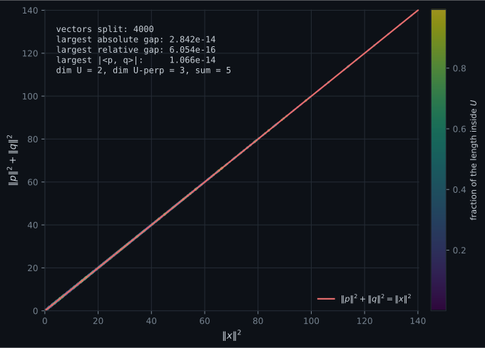
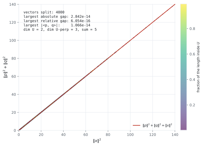
Reading the plot

From the Pythagoras scatter. The colour is doing real work. It runs from dark (almost none of the vector’s length is inside $U$) to bright (almost all of it is), so the sample is not concentrated on some convenient middle case. Every one of the four thousand points sits on the diagonal regardless, and the largest relative deviation is $6.054\times10^{-16}$.

The other measured column is the one to remember: $\lvert\langle\mathbf{p},\mathbf{q}\rangle\rvert$ peaks at $1.066\times10^{-14}$. The cross term is what has to vanish for Pythagoras, and it does — which is the only reason the two squared parts add up. Split a vector along two non-perpendicular directions and the squares do not add.

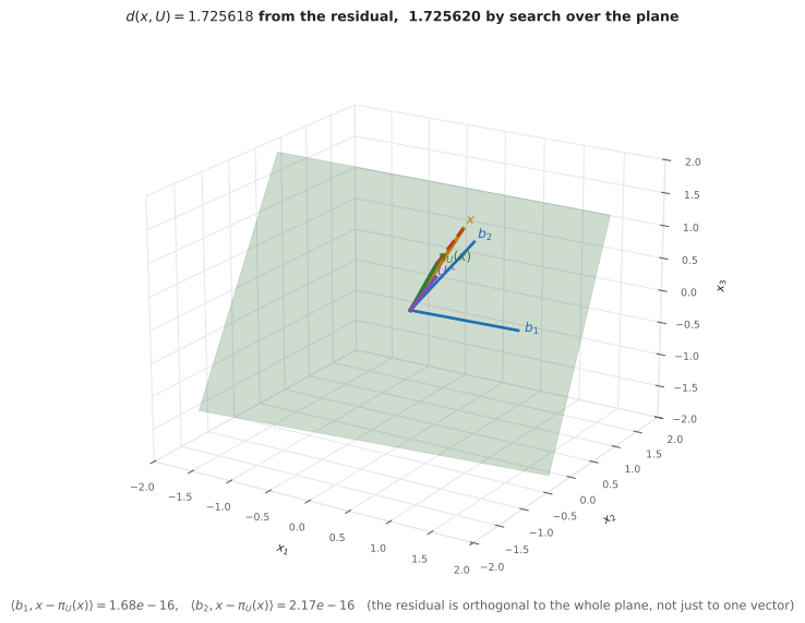
From the three-dimensional plane. The measured distance from the residual is $1.725618$ and the brute-force scan over a $1201 \times 1201$ grid gives $1.725620$. The disagreement is in the sixth decimal and it is the grid’s fault, not the formula’s: with a spacing of $0.005$ over the plane, the nearest sampled point cannot be closer than the true foot. The closed form is exact; the search is the approximation. That ordering is easy to get backwards.

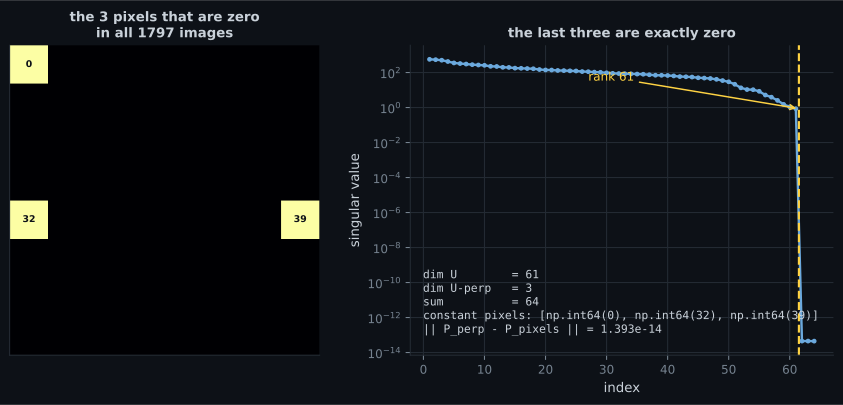
From the pixel grid. This is the figure to keep. The centred digit matrix has rank $61$ in $64$ dimensions, so its orthogonal complement is exactly $3$-dimensional — and that complement is not an abstract three-dimensional thing, it is the span of the coordinate axes of pixels 0, 32 and 39. The comparison is measured: $\lVert \mathbf{P}_{U^\perp} - \mathbf{P}_{\text{pixels}}\rVert = 1.393\times10^{-14}$.

Those three pixels are zero in all $1797$ images. Any direction that only moves them takes you nowhere the data can go, which is precisely what “in the orthogonal complement of the data” means. The abstract statement $\dim U + \dim U^\perp = D$ here reads $61 + 3 = 64$, and every term is countable.

It also explains the arithmetic on the Basis and Rank page from the other direction: the rank is $61$ because three pixels never vary, and $64 - 3 = 61$.

Pitfalls

The complement depends on the inner product, so whitening moves it

$U^\perp$ is defined by $\langle\mathbf{v},\mathbf{u}\rangle = 0$, and that inner product is a choice. Under $\langle\mathbf{x},\mathbf{y}\rangle = \mathbf{x}^\top\mathbf{A}\mathbf{y}$ the complement is the null space of $\mathbf{B}^\top\mathbf{A}$, not of $\mathbf{B}^\top$. So the “discarded directions” of a PCA on raw features and a PCA on whitened features are different subspaces, not the same subspace in different coordinates.

Orthogonal complement is not set complement

$U^\perp$ is not “everything not in $U$”. It is a subspace, it contains $\mathbf{0}$, and it is much smaller than the set-theoretic complement — a line’s orthogonal complement in $\mathbb{R}^3$ is a plane, while the set of vectors not on the line is almost all of $\mathbb{R}^3$. The relationship is $U \oplus U^\perp = V$ (a direct sum), not $U \cup U^\perp = V$.

Rank determination decides the dimension, and it needs a tolerance

complement_basis above counts singular values above sv.max() * n * eps. Change that threshold and the reported dimension of $U^\perp$ changes. On the digit data the gap is unambiguous — the last three singular values are exactly $0$ while the smallest nonzero one is $0.860$ — but on noisy data there is no gap, and “the dimension of the complement” becomes a modelling decision rather than a fact. This is the same tolerance question as on the Basis and Rank page.

Pythagoras needs the two parts to be orthogonal, not merely different

$\lVert\mathbf{x}\rVert^2 = \lVert\mathbf{p}\rVert^2 + \lVert\mathbf{q}\rVert^2$ holds because $\langle\mathbf{p},\mathbf{q}\rangle = 0$. Any other decomposition $\mathbf{x} = \mathbf{p}' + \mathbf{q}'$ — an oblique projection, a non-orthogonal factor split — has a nonzero cross term, and then “the share of the variance explained by this component” does not add up to $100\%$. Factor analysis with oblique rotations has exactly this property, which is why its loadings are not squared and summed.

A one-dimensional complement gives a normal vector up to sign and scale

$\mathbf{w}$ and $-3\mathbf{w}$ describe the same hyperplane. Any code that stores a normal vector has to fix a convention (unit length and, say, a positive first nonzero entry) or two runs will disagree about the orientation of the same plane. np.cross and np.linalg.svd both make arbitrary sign choices.

Compare

object	dimension	how it is specified	what it is used for
subspace $U$	$M$	$M$ spanning vectors	the part you keep
complement $U^\perp$	$D - M$	$D-M$ spanning vectors, or the null space of $U$‘s basis	the part you discard: residuals, reconstruction error
hyperplane	$D-1$	one normal vector	decision boundaries (Ch 12)
line	$1$	one direction vector	one principal component
projector onto $U$	rank $M$	$\mathbf{Q}\mathbf{Q}^\top$ for orthonormal $\mathbf{Q}$	§3.8
projector onto $U^\perp$	rank $D-M$	$\mathbf{I} - \mathbf{Q}\mathbf{Q}^\top$	residual maker

The last row is worth memorising: the residual operator is one minus the projector, and its rank is the complement’s dimension. It appears in every least-squares derivation in Chapter 9.

pch.quizTag Check your understanding

1. Why is the decomposition x = p + q into a U-part and a U-perp-part unique?

   A Because projections are linear B Because U and U-perp share only the zero vector — if there were two decompositions, their difference would be a nonzero vector lying in both subspaces at once C Because U-perp is one-dimensional D It is not unique in general
   pch.quizShowAnswer

   B — Because U and U-perp share only the zero vector — if there were two decompositions, their difference would be a nonzero vector lying in both subspaces at once — And the trivial intersection itself comes from positive definiteness: a vector in both is orthogonal to itself, so its inner product with itself is zero, so it is the zero vector.

2. The centred digit matrix has rank 61 in 64 pixel dimensions. What is its orthogonal complement?

   A An abstract three-dimensional subspace with no concrete description B The span of the coordinate axes of pixels 0, 32 and 39 — the three that are zero in all 1797 images, verified by comparing the two projectors, which differ by 1.4e-14 C The set of all images not in the dataset D Empty, since the matrix has full rank
   pch.quizShowAnswer

   B — The span of the coordinate axes of pixels 0, 32 and 39 — the three that are zero in all 1797 images, verified by comparing the two projectors, which differ by 1.4e-14 — The dimension count reads 61 + 3 = 64 with every term countable. It is also the reason the rank is 61 rather than 64 in the first place.

3. The brute-force grid search finds a distance of 1.725620 where the closed form gives 1.725618. Which is more accurate?

   A The grid search, since it makes no assumptions B The closed form. A grid over the plane cannot land exactly on the foot of the perpendicular, so a search can only ever overestimate — the sixth-decimal difference is the grid spacing, not formula error C Neither; they disagree so both are suspect D They are equally accurate
   pch.quizShowAnswer

   B — The closed form. A grid over the plane cannot land exactly on the foot of the perpendicular, so a search can only ever overestimate — the sixth-decimal difference is the grid spacing, not formula error — The grid spacing is 0.005 over the plane. Getting the direction of this bias backwards is a common way to distrust a correct formula.

4. Which statement about the orthogonal complement is wrong?

   A It is a subspace, so it contains the zero vector B Its dimension is D minus the dimension of U C It is the set of all vectors not in U D Checking orthogonality against a basis of U is enough to be orthogonal to all of U
   pch.quizShowAnswer

   C — It is the set of all vectors not in U — Orthogonal complement is not set complement. A line's complement in three dimensions is a plane, whereas the set of vectors not on the line is nearly all of the space. The correct relationship is a direct sum: U plus U-perp equals V.

🧪 Try It Yourself

Exercise 1 – Find a complement basis

pch.exerciseTag pch.exerciseTitle

Exercise 2 – Verify Pythagoras 4000 times

pch.exerciseTag pch.exerciseTitle

Exercise 3 – Break Pythagoras with an oblique split

pch.exerciseTag pch.exerciseTitle

Exercise 4 – Identify the digits complement

pch.exerciseTag pch.exerciseTitle

Exercise 5 – The residual operator

pch.exerciseTag pch.exerciseTitle

Recall card

• The orthogonal complement is every vector orthogonal to all of U, and it is a subspace rather than a set, because orthogonality to a fixed vector is a linear condition.
• Its dimension is D minus the dimension of U, and the two subspaces share only the zero vector — which follows from positive definiteness, since a vector in both is orthogonal to itself.
• Checking orthogonality against a basis of U suffices, so the complement is the null space of the matrix whose rows are that basis.
• Every vector splits uniquely into a U part and a U-perp part, Equation 3.36.
• Pythagoras holds for that split because the cross term is zero. Measured over four thousand vectors in five dimensions, the largest relative gap was six times ten to the minus sixteen.
• A codimension-one subspace is described by a single normal vector, and the distance from a point to it is the absolute inner product divided by the normal’s length — which is the basis of the support vector machine in Chapter 12.
• The residual operator is one minus the projector; it is itself a projector, its rank is the complement’s dimension, and its trace equals its rank.
• The handwritten-digit data has rank 61 of 64, and its orthogonal complement is exactly the span of the three pixel axes that are zero in every image.

Next: Inner Product of Functions — the same definitions, with the sum replaced by an integral.