What you’ll learn

• the decomposition $\mathbb{E}[(y - \hat{f})^2] = \text{bias}^2 + \text{variance} + \sigma^2$, derived line by line
• what the expectation is taken over, which is the part that confuses everyone
• the three terms computed by hand from four numbers
• the same three terms measured by simulation across model capacity
• why the third term is a hard floor, and how to estimate it
• why “tradeoff” is slightly the wrong word for modern models

Intuition

Underfitting vs Overfitting diagnosed two failures from measurements. This page explains why there are exactly two, and where a third, unfixable source of error comes from.

The thought experiment: imagine training your model not once but a thousand times, each on a fresh sample from the same source. You now have a thousand models, and at any input $x_0$ a thousand predictions. Two things can be wrong with that cloud of predictions:

• Bias — the cloud is centred in the wrong place. Every model makes the same mistake.
• Variance — the cloud is spread out. The models disagree with each other.

And one thing is wrong with the target rather than the models: noise. Even a perfect model cannot predict the part of $y$ that is not a function of $x$.

figureFifty models per panel, each trained on its own samplematplotlib

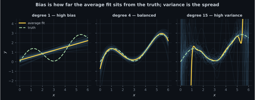
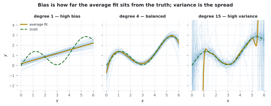
That figure is the decomposition, drawn. Left panel: amber sits well away from green (high bias) and the blue lines are tight (low variance). Right panel: amber tracks green (low bias) and the blue lines are everywhere (high variance).

The math

Setup

The data is generated by an unknown function plus noise:

You fit $\hat{f}$ on a training set $D$. Because $D$ is a random sample, $\hat{f}$ is itself random. Fix an input $\mathbf{x}_0$ and ask for the expected squared error there, averaged over both the noise and the choice of training set:

That double expectation is the whole subtlety. You never observe it — you have one training set — but it is what “how good is this modelling approach” means.

Derivation

Write $\bar{f}(\mathbf{x}_0) = \mathbb{E}_D[\hat{f}_D(\mathbf{x}_0)]$ for the average prediction across training sets. Add and subtract it inside the square:

Square, and take the expectation of all nine terms. Every cross term vanishes:

• $\mathbb{E}[\varepsilon] = 0$ and $\varepsilon$ is independent of $D$, so both cross terms involving $\varepsilon$ are zero.
• $\mathbb{E}_D[\bar{f} - \hat{f}] = 0$ by the definition of $\bar{f}$, and $(f - \bar{f})$ is a constant with respect to $D$, so their cross term is zero too.

What remains is three squares:

Three non-negative terms. Two you control, one you do not.

Worked example by hand

You train the same model on four different samples. At one input $\mathbf{x}_0$, the four predictions are:

The true value is $f(\mathbf{x}_0) = 6$, and the noise has $\sigma^2 = 1$.

Step 1 — the average prediction.

Step 2 — bias.

Step 3 — variance.

Step 4 — total expected error.

Step 5 — verify directly. Compute the mean squared distance from each prediction to the true $f$, then add the noise term:

The two routes agree, and $4.5 = 1 + 3.5$ confirms the decomposition exactly. Note what it says about this model: variance (3.5) is three and a half times bias² (1), so the problem is instability, not systematic error. Simplify or average, do not add capacity.

Measuring it

You cannot compute this on real data — you have one training set and you do not know $f$. On simulated data you know both, so the terms can be measured directly.

figure200 training sets per degree, three terms measuredmatplotlib

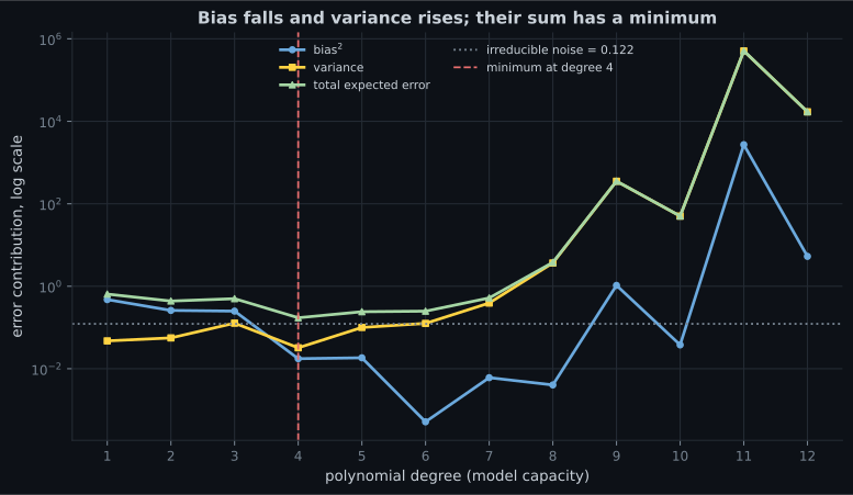
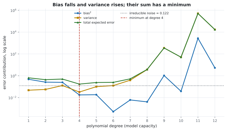
Measured with 200 simulated training sets of 30 points each, $\sigma = 0.35$ so $\sigma^2 = 0.1225$:

Reading the plot

1. Bias falls fast, then stops. From 0.474 at degree 1 to 0.017 at degree 4 — a 96% reduction. Past that there is nothing left to remove, and degree 8 only improves it to 0.006.
2. Variance is quiet, then explodes. Flat around 0.05 up to degree 4, then 1.43 by degree 8 — a thirtyfold jump for two extra degrees.
3. The minimum is where the curves cross in importance, not where either is smallest.
4. Degree 12 is a numerical artefact worth noticing. Bias² rises to 32, which the theory says should not happen — more capacity cannot increase bias. What actually happened is that fitting a degree-12 polynomial to 30 points is so ill-conditioned that the fits are numerically garbage, so even their average is wild. Real instability, showing up in a term that should be monotone.

import numpy as np
 
TRUE = lambda x: np.sin(1.5 * x) + 0.35 * x
NOISE = 0.35
x_eval = np.linspace(0, 6, 200)
truth = TRUE(x_eval)
 
rng = np.random.default_rng(1)
 
for degree in (1, 2, 4, 8):
    predictions = np.empty((200, len(x_eval)))
    for run in range(200):
        x = rng.uniform(0, 6, 30)
        y = TRUE(x) + rng.normal(0, NOISE, 30)
        predictions[run] = np.polyval(np.polyfit(x, y, degree), x_eval)
 
    mean_prediction = predictions.mean(axis=0)
    bias_squared = float(((mean_prediction - truth) ** 2).mean())
    variance = float(predictions.var(axis=0).mean())
    total = bias_squared + variance + NOISE**2
 
    print(f"degree {degree:2d}  bias^2 {bias_squared:8.4f}  "
          f"variance {variance:8.4f}  total {total:8.4f}")
 
# degree  1  bias^2   0.4743  variance   0.0474  total   0.6442
# degree  2  bias^2   0.2593  variance   0.0559  total   0.4377
# degree  4  bias^2   0.0168  variance   0.0461  total   0.1854
# degree  8  bias^2   0.0056  variance   1.4330  total   1.5611

import numpy as np
 
TRUE = lambda x: np.sin(1.5 * x) + 0.35 * x
NOISE = 0.35
x_eval = np.linspace(0, 6, 200)
truth = TRUE(x_eval)
 
rng = np.random.default_rng(1)
 
for degree in (1, 2, 4, 8):
    predictions = np.empty((200, len(x_eval)))
    for run in range(200):
        x = rng.uniform(0, 6, 30)
        y = TRUE(x) + rng.normal(0, NOISE, 30)
        predictions[run] = np.polyval(np.polyfit(x, y, degree), x_eval)
 
    mean_prediction = predictions.mean(axis=0)
    bias_squared = float(((mean_prediction - truth) ** 2).mean())
    variance = float(predictions.var(axis=0).mean())
    total = bias_squared + variance + NOISE**2
 
    print(f"degree {degree:2d}  bias^2 {bias_squared:8.4f}  "
          f"variance {variance:8.4f}  total {total:8.4f}")
 
# degree  1  bias^2   0.4743  variance   0.0474  total   0.6442
# degree  2  bias^2   0.2593  variance   0.0559  total   0.4377
# degree  4  bias^2   0.0168  variance   0.0461  total   0.1854
# degree  8  bias^2   0.0056  variance   1.4330  total   1.5611

See it move

The classic dartboard. Each panel is a different model, each dart a different training set. Bias is how far the cluster sits from the bullseye; variance is how wide the cluster is.

The irreducible term

$\sigma^2$ is the variance of $y$ given $\mathbf{x}$ — the part of the target that the features simply do not determine. Two identical districts can sell for different prices; two patients with identical charts can have different outcomes.

No model reduces it. A reported error below $\sigma^2$ is not a triumph, it is evidence of a leak or of evaluating on training data.

You can estimate it, though: fit a very flexible model with plenty of data and see where the validation error plateaus. That floor is roughly $\sigma^2$, and it tells you when to stop investing in the model and start investing in better features — because more features are the only thing that reduces $\sigma^2$. Adding a column that genuinely explains part of the leftover variation moves the floor down; nothing else does.

What moves each term

The last two rows are why Phase 5 exists. Bagging averages many high-variance, low-bias models and cancels the variance; boosting combines many high-bias, low-variance models and cancels the bias. Both are direct applications of this decomposition rather than clever tricks.

Diagnosing from two numbers

You cannot measure bias and variance separately on real data, but the pair (training error, validation error) tells you which term dominates — and that is enough to choose the next action:

  flowchart TD
  A["Fit the model.
Record training error
and validation error."] --> B{"Training error
already high?"}
  B -->|"yes -- underfits its own data"| C["Bias dominates"]
  C --> D["Add capacity, add informative
features, reduce regularisation.
More data will NOT help."]
  B -->|"no -- fits training data well"| E{"Big gap between
training and validation?"}
  E -->|"yes, gap is large"| F["Variance dominates"]
  F --> G["More data, more regularisation,
bagging, early stopping,
fewer noise features."]
  E -->|"no, both errors close
and both acceptable"| H{"Is validation error
near the estimated floor?"}
  H -->|"yes"| I["You are at sigma squared.
Only new features move it.
Stop tuning."]
  H -->|"no, and neither error
is improving"| J["Re-check the target,
the split, and the metric
before touching the model."]
  D --> A
  G --> A

The loop matters as much as the branches: every action changes the two numbers, so the diagnosis has to be repeated rather than made once. The costly mistake is taking the “variance” action — collect more data — while sitting in the “bias” branch, where more data changes nothing at all.

Pitfalls

🧪 Try It Yourself

Exercise 1 – Decompose four predictions

Exercise 2 – Verify the decomposition

Exercise 3 – Measure both terms by simulation

Exercise 4 – Watch averaging kill variance

Exercise 5 – Find the noise floor

Recap

• $\text{Err} = \text{bias}^2 + \text{variance} + \sigma^2$, exactly, with every cross term vanishing.
• The expectation is over the noise and the random training set — variance only exists because the model is itself a random object.
• Hand-worked: predictions 3, 5, 4, 8 against a truth of 6 give bias² 1, variance 3.5, total 5.5, and both routes agree.
• Measured: bias² falls 0.474 → 0.017 by degree 4, while variance rises 0.046 → 1.433 by degree 8. The minimum total is at degree 4.
• $\sigma^2$ is a floor. Only better features move it; no model does.
• Bagging attacks variance, boosting attacks bias, and both come directly from this decomposition.

Exercise 6 – Decompose the error, empirically

Next

Continue to K-Fold Cross-Validation — the practical machinery for estimating held-out error without the thousand training sets this page assumed.