How Neural Networks Learn (Gradient-Based Optimization)

Training is one line repeated: move every parameter a little way against its gradient. Everything interesting is in “a little way” — this page derives the exact ceiling on the step size, then measures what happens at five learning rates and five batch sizes.

What you’ll learn

• The update rule, with one SGD step reproduced by hand to 0.00e+00 against Keras.
• Why the stability limit is $2/\text{curvature}$ — derived, then tested at four rates.
• A learning-rate sweep spanning 0.1320 to 0.8960 validation accuracy on identical models, and why lr=1.0 did not explode here.
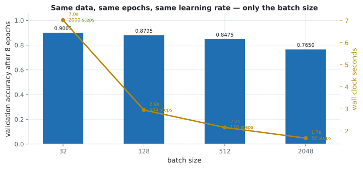
• What batch size buys: batch 32 reached 0.9005 in 6.5s, batch 2048 0.7650 in 1.7s, and batch 8 took 34 minutes.
• Why anisotropic curvature makes one learning rate wrong for two parameters.
• A case where plain SGD beat both momentum and Adam by three orders of magnitude.

The update rule

For every parameter $\theta_i$ and a loss $L$:

$$\theta_i \leftarrow \theta_i - \eta \frac{\partial L}{\partial \theta_i}$$

The gradient points in the direction of steepest increase, so subtracting it decreases the loss. $\eta$ (the learning rate) sets how far you commit to that direction.

diagram Diagram mermaid

  flowchart LR
  B["one mini-batch"] --> F["forward pass:
predictions"]
  F --> L["loss:
one number"]
  L --> G["backward pass:
dL/dtheta for every parameter"]
  G --> U["theta = theta - eta * gradient"]
  U --> B
  N["one pass over every batch = one epoch"] -.-> B

Verified against Keras on a single sigmoid unit, one row, $\eta = 0.5$:

	Value
prediction	0.093652
loss (binary cross-entropy)	2.368167
$\partial L/\partial \mathbf{W}$	[−0.906348, −0.453174, +0.453174, −1.812696]
$\mathbf{W}$ after a manual step	[0.487537, −0.191737, 0.515915, 0.044456]
$\mathbf{W}$ after SGD.apply_gradients	[0.487537, −0.191737, 0.515915, 0.044456]
difference	0.00e+00

An optimiser is that subtraction plus bookkeeping. Note the third gradient component is the only positive one — its input was the only negative feature.

How large a step is too large?

Take $L(w) = (w - 1)^2$ and write out one step:

$$w' = w - \eta \cdot 2(w-1) \quad\Longrightarrow\quad (w' - 1) = (1 - 2\eta)(w - 1)$$

The distance to the minimum is multiplied by $\lvert 1 - 2\eta \rvert$ every step, which gives the entire picture:

• $\lvert 1 - 2\eta\rvert < 1$ — converges, requiring $0 < \eta < 1$.
• $\eta = 0.5$ — the factor is 0: it lands exactly on the minimum in one step.
• $\eta = 1$ — the factor is $-1$: it bounces between two points forever.
• $\eta > 1$ — the factor exceeds 1 and the distance grows.

For curvature $c$ (the second derivative) the limit is $\eta < 2/c$. Tested:

$\eta$	Final loss after 30 steps	Behaviour
0.4	0.0000e+00	converges
0.9	1.3792e−05	converges, oscillating
1.0	9.0000e+00	bounces forever, never improves
1.1	5.0713e+05	diverges

At $\eta = 0.3$ the factor is 0.4, so each step leaves 40% of the distance:

Step	$w$	Loss	Gradient
0	4.000000	9.000000	6.000000
1	2.200000	1.440000	2.400000
2	1.480000	0.230400	0.960000
3	1.192000	0.036864	0.384000
4	1.076800	0.005898	0.153600
5	1.030720	0.000944	0.061440

When the curvature differs by axis

Real losses are not symmetric bowls. For $L(a,b) = a^2 + 10b^2$ the curvature is 2 along $a$ and 20 along $b$, so the stability limits are 1.0 and 0.1. One learning rate must satisfy the tightest axis.

figure The same bowl, three step sizes matplotlib

Starting loss 16.8. lr=0.02 reaches 0.258 in 40 steps — stable but slow along the flat axis. lr=0.09 reaches 1.04e-06, zig-zagging because it is just under the b-axis limit of 0.1. lr=0.101 is just past that limit and the loss grows to 48.8.

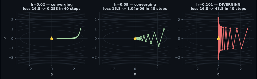
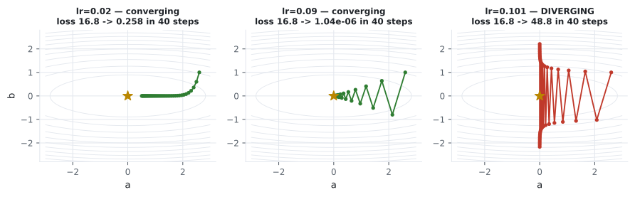
$\eta$	Loss: start → after 40 steps
0.02	16.8 → 0.258	converging, slowly
0.09	16.8 → 1.038e−06	converging, zig-zagging
0.101	16.8 → 48.75	diverging

A condition number of 10 — mild by real standards — already forces a compromise: fast enough for $a$ is unstable for $b$. This is why feature scaling matters, why the MLP page’s weights received gradients proportional to their inputs, and why Phase 2’s normalisation layers exist.

What the learning rate does to a real model

Identical model, identical seed, plain SGD, 15 epochs on 8,000 MNIST rows:

figure Five learning rates, everything else held fixed matplotlib

lr=0.0001 is not broken, just a thousand times too slow — after 15 epochs it reached 0.1320, barely above the 0.10 of guessing. lr=1.0 did not diverge on this problem; it matched lr=0.1 almost exactly. The useful range spans two orders of magnitude.

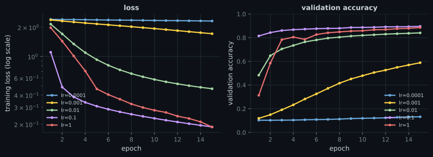
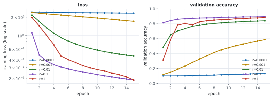
Learning rate	Final training loss	Final validation accuracy
0.0001	2.318552	0.1320
0.001	1.714472	0.5885
0.01	0.464704	0.8405
0.1	0.187716	0.8960
1.0	0.187320	0.8855

Two honest readings. A learning rate 1,000× too small looks exactly like a broken model — 0.1320 accuracy and a loss that barely moves. Sweep the rate before suspecting the architecture. And lr=1.0 did not explode, which the textbook picture would predict. Cross-entropy on this shallow ReLU network has gentle enough curvature that a step of 1.0 stayed inside the limit. Theory gives you $2/c$; only measurement tells you what $c$ is.

Batch size: more steps against cheaper steps

figure Same data, same epochs, same learning rate — only the batch size matplotlib

Batch 32 takes 2,000 steps and 6.5 seconds to reach 0.9005; batch 2048 takes 32 steps and 1.7 seconds to reach 0.7650. Holding epochs fixed while changing the batch size changes the number of updates by 62x, so this compares update counts as much as batch sizes.

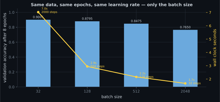
Batch size	Steps (8 epochs)	Seconds	Validation accuracy
8	8,000	2,047.93	0.9245
32	2,000	6.49	0.9005
128	504	3.05	0.8795
512	128	2.02	0.8475
2048	32	1.69	0.7650

The batch-8 row was measured once and deliberately left out of the figure build: 34 minutes to buy 0.0240 accuracy over batch 32’s 6.5 seconds — a 315× time cost for a 2.7% relative gain. That is why batch sizes of 32–512 dominate in practice.

Note what this does not show. Holding epochs fixed gave the small-batch runs 62× more updates, so part of their advantage is simply more optimisation. A fair batch-size experiment fixes the step count and scales the learning rate — which is what Phase 8 does when it measures throughput properly.

Mini-batch SGD, written out

$$\theta \leftarrow \theta - \eta \cdot \frac{1}{|B|}\sum_{i \in B} \nabla_\theta L_i$$

The batch average is what makes the gradient usable: one example’s gradient is a very noisy estimate of the full-dataset gradient, and the full dataset is too expensive to evaluate every step. Mini-batches are the compromise, and the tensor page’s throughput measurement — 61 GFLOP/s at n=64 against 199 at n=1024 — is why a batch is processed as one matmul rather than a loop.

Momentum and Adam, and where they help

Momentum keeps a running velocity, so consistent directions accumulate:

$$v \leftarrow \beta v + \nabla_\theta L, \qquad \theta \leftarrow \theta - \eta v$$

Adam additionally divides each parameter’s step by a running estimate of its own gradient magnitude, which directly attacks the per-axis curvature problem above.

On the anisotropic bowl, 60 steps at $\eta = 0.05$:

Optimiser	Final loss
plain SGD	2.182971e−05
SGD + momentum 0.9	1.910986e−02
Adam	9.709373e−02

Plain SGD won by three orders of magnitude. On a clean two-parameter quadratic with a well-chosen rate there is nothing for momentum to accelerate and nothing for Adam to rescale, so their extra state only overshoots. Adam earns its default-choice status on messy, high-dimensional, non-stationary losses — not on this. Phase 2 compares them where the difference goes the other way, which is the honest place to do it.

See it move

sketch A ball descending a loss surface p5.js Pause Restart

The white ball starts high on the loss curve and steps downhill each frame, using the local slope (gradient) to decide which way to move -- then eases back to the start and does it again.

The second sketch is the stability limit you can feel. Drag the rate past $2/c$ and the path stops converging — the boundary sits exactly where the algebra says it does.

sketch Cross the stability limit yourself p5.js Pause Restart

Gradient descent on a quadratic with draggable learning rate and curvature. The convergence factor is shown live: below 1 the path converges, at exactly 1 it bounces forever, above 1 it diverges.

Pitfalls

Diagnosing a too-small learning rate as a bad architecture. lr=0.0001 gave 0.1320 accuracy — indistinguishable from a broken model. Sweep the rate first; it costs five short runs.

Assuming a large learning rate always diverges. lr=1.0 matched lr=0.1 here. The limit is $2/c$, and you do not know $c$ until you measure.

Comparing batch sizes at a fixed epoch count. That changes the update count by 62× between batch 32 and 2048, so two variables move at once.

Using a tiny batch to “learn better”. Batch 8 cost 2,047.93s against batch 32’s 6.49s for 0.0240 more accuracy.

Reaching for Adam automatically. On this well-conditioned problem plain SGD beat it by three orders of magnitude. Adam is a good default on hard problems, not a strictly better algorithm.

Forgetting the gradient is a batch average. Changing the batch size changes the gradient’s variance, which interacts with the learning rate — they are not independent knobs.

Recap

• $\theta \leftarrow \theta - \eta\,\partial L/\partial\theta$, reproduced by hand to 0.00e+00 against SGD.apply_gradients.
• For $(w-1)^2$, one step multiplies the distance to the minimum by $\lvert 1 - 2\eta\rvert$; in general $\eta < 2/c$. Tested: 0.9 converges, 1.0 bounces forever, 1.1 diverges to 5.07e+05.
• Anisotropic curvature forces a compromise — on $a^2 + 10b^2$ the limits are 1.0 and 0.1, so 0.101 diverged while 0.09 converged to 1.04e−06.
• On real data: 0.1320 accuracy at lr=0.0001 against 0.8960 at lr=0.1, and lr=1.0 did not diverge.
• Batch size: 32 → 0.9005 in 6.49s, 2048 → 0.7650 in 1.69s, 8 → 0.9245 in 2,047.93s.
• Plain SGD beat momentum and Adam on the clean quadratic; their advantage lies on messy losses.

pch.quizTag pch.quizDefaultTitle

1. Your model trains 15 epochs and reaches 0.1320 validation accuracy on a 10-class problem. What should you check first?

   A The architecture — it is clearly too small B The learning rate. Measured here, lr=0.0001 produced exactly that, while lr=0.1 on the identical model and seed reached 0.8960 C The label encoding D Whether the data is shuffled
   pch.quizShowAnswer

   B — The learning rate. Measured here, lr=0.0001 produced exactly that, while lr=0.1 on the identical model and seed reached 0.8960 — A rate three orders of magnitude too small is indistinguishable from a broken model. A log-spaced sweep of five short runs is the cheapest diagnostic in deep learning.

2. For L(w) = (w-1)², what happens at exactly eta = 1.0?

   A It converges fastest B The distance to the minimum is multiplied by |1 - 2| = 1 every step, so it bounces between two points forever — measured, the loss was still 9.0000 after 30 steps C It diverges immediately D It lands on the minimum in one step
   pch.quizShowAnswer

   B — The distance to the minimum is multiplied by |1 - 2| = 1 every step, so it bounces between two points forever — measured, the loss was still 9.0000 after 30 steps — eta = 0.5 is the rate that lands exactly on the minimum (factor 0). Convergence needs the factor below 1, meaning eta < 1 here and eta < 2/c in general.

3. On L(a,b) = a² + 10b², why can one learning rate not suit both parameters?

   A Because b has a larger coefficient B The curvatures are 2 and 20, so the limits are 1.0 and 0.1 — anything fast enough for a is unstable for b; measured, 0.101 diverged while 0.09 converged C Because gradient descent needs symmetric losses D It can, with enough steps
   pch.quizShowAnswer

   B — The curvatures are 2 and 20, so the limits are 1.0 and 0.1 — anything fast enough for a is unstable for b; measured, 0.101 diverged while 0.09 converged — A condition number of 10 is mild and already forces the compromise. This is the mechanism behind feature scaling, normalisation layers and per-parameter optimisers.

4. Batch 32 reached 0.9005 and batch 2048 reached 0.7650 after the same 8 epochs. What is the flaw in concluding small batches generalise better?

   A There is none — the result is clear B At fixed epochs, batch 32 took 2,000 updates against batch 2048's 32 — a 62x difference, so the comparison conflates batch size with the amount of optimisation C The batch sizes are too far apart D Validation accuracy is the wrong metric
   pch.quizShowAnswer

   B — At fixed epochs, batch 32 took 2,000 updates against batch 2048's 32 — a 62x difference, so the comparison conflates batch size with the amount of optimisation — To isolate batch size you fix the step count and scale the learning rate. As run here, much of the gap is simply that the small-batch model took far more updates.

5. Plain SGD finished at 2.18e-05 while Adam finished at 9.71e-02 on the same bowl. What does that tell you?

   A Adam is a worse optimiser B That on a clean low-dimensional problem with a well-chosen rate there is nothing for Adam's adaptive scaling to fix, so its extra state only overshoots — its advantage appears on messy high-dimensional losses C The Adam implementation is buggy D Adam needs a warm-up
   pch.quizShowAnswer

   B — That on a clean low-dimensional problem with a well-chosen rate there is nothing for Adam's adaptive scaling to fix, so its extra state only overshoots — its advantage appears on messy high-dimensional losses — Benchmarks decide optimisers, not reputations. Adam is the right default when you cannot tune a rate per problem, which is the usual situation — but not this one.

Next

You know the update rule and its hard limit. Continue to Building Neural Networks with Keras to assemble models the framework way, or to Autograd from Scratch to see where these gradients come from.

🧪 Try It Yourself

Exercise 1 – Descend a one-parameter loss

pch.exerciseTag pch.exerciseTitle

Exercise 2 – Find the stability limit

pch.exerciseTag pch.exerciseTitle

Exercise 3 – One rate, two curvatures

pch.exerciseTag pch.exerciseTitle

Exercise 4 – Reproduce one SGD step

pch.exerciseTag pch.exerciseTitle

Exercise 5 – Count the updates

pch.exerciseTag pch.exerciseTitle

Exercise 6 – SGD, momentum and Adam on the same bowl

pch.exerciseTag pch.exerciseTitle