Limitations and the Future of Deep Learning

A closing chapter on what deep learning cannot do is usually an essay. It does not have to be. Each of the classic limitations is a claim about a model’s behaviour, and every one of them can be measured on a model you have just trained.

So here is one: a 225,034-parameter convnet at 0.9785 accuracy on held-out MNIST. Below is what it does when the world moves slightly.

Change	Accuracy	Its confidence
None	0.9785	0.9821
Shifted 4 pixels diagonally	0.0975	0.7729
Rotated 45°	0.4800	0.7977
Colours inverted	0.1705	0.7940
Adversarial noise, ε = 0.2	0.3250	0.8035
Random noise, ε = 0.2	0.9850	—

Every one of those failures is confident. The model does not signal distress, produce a low probability, or refuse to answer — it returns a wrong label at roughly 0.78 confidence, which is the single most important fact on this page.

What you’ll learn

Why a convolutional network is not shift-invariant, despite what the intuition suggests.
Why adversarial noise destroys a model that identical-magnitude random noise leaves untouched.
What the learning curve says about the cost of the next decimal place — measured, then extrapolated.
Why “confidence” is not a usable uncertainty estimate, in four separate experiments.

Local generalisation

figure 2,000 held-out digits, transformed after training matplotlib

The shift curve is the surprising one: two pixels costs 0.2195 and four pixels costs 0.8810, leaving the model below random guessing. A human reading these digits would not notice a four-pixel shift on a 28-pixel canvas. Contrast, by contrast, barely matters — 0.9610 at quarter contrast — because scaling every pixel is close to a transformation the first convolution can absorb.

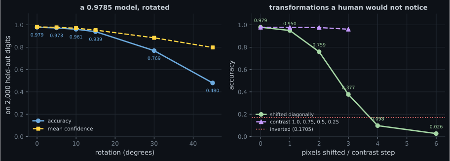
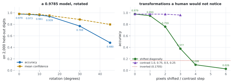
Shift	Accuracy	Rotation	Accuracy
0 px	0.9785	0°	0.9785
1 px	0.9495	5°	0.9725
2 px	0.7590	15°	0.9390
3 px	0.3770	30°	0.7690
4 px	0.0975	45°	0.4800

Why shifting breaks a convnet

Convolution is translation-equivariant: shift the input and the feature map shifts with it. That is not the same as translation-invariant, which is what classification needs. The Flatten layer destroys the distinction — it maps each spatial position to a fixed set of dense weights, so a feature that has moved four pixels now multiplies entirely different parameters.

Pooling buys back a little tolerance (two MaxPooling2D layers here, hence surviving one pixel at 0.9495) and no more. Invariance to a transformation comes from the training data, or from an architecture built for it — never for free. Train with random shifts and this curve flattens; that is exactly what data augmentation buys, and why it is not optional in vision.

The inverted-colour result makes the same point differently. Nothing in a convnet knows that brightness is not semantic. It scored 0.1705 on images a human reads instantly.

Adversarial fragility

Left: accuracy against perturbation size for adversarial and random noise. The adversarial curve falls from 0.9850 to 0.3250 while the random-noise curve stays flat at 0.9850, with confidence under attack falling only to 0.8035. Right: three images side by side — a clean digit, the attacked version which looks nearly identical, and their difference amplified five times. — At epsilon 0.2 the adversarial direction takes accuracy to 0.3250 while random noise of the same magnitude leaves it at 0.9850 — completely unchanged. That contrast is the entire result: this is not sensitivity to noise, it is sensitivity to one specific direction out of 784, and the mean pixel change of 0.0923 is small enough that the two images look the same.

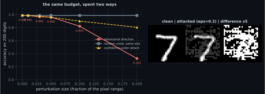
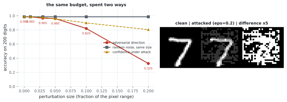
The attack is a single line of the same calculus used to train the model:

Fast gradient sign, in full

with tf.GradientTape() as tape:
    tape.watch(images)
    loss = loss_function(labels, model(images, training=False))
 
direction = np.sign(tape.gradient(loss, images).numpy())
attacked = np.clip(images + epsilon * direction, 0, 1)

Gradient ascent on the loss — the same tool as DeepDream, aimed at making the model wrong instead of making a layer excited.

ε	Adversarial	Random noise	Mean pixel change
0.05	0.9600	0.9850	0.0237
0.10	0.8200	0.9850	0.0468
0.20	0.3250	0.9850	0.0923

The random-noise column is what makes this interpretable. A model that degraded under both would merely be noise-sensitive. This one is untouched by random perturbation and destroyed by a perturbation of the same size pointed in one particular direction — which means the decision boundary passes far closer to every training point than its accuracy suggests.

The cost of the next decimal place

Left: accuracy against training-set size on a log axis, rising from 0.6645 at 250 examples to 0.9785 at 12,000. Right: the same data as error rate on log-log axes, falling in a nearly straight line, with a fitted power law of exponent -0.690. — A straight line on log-log axes is a power law, and this one has exponent -0.690: error falls as roughly the inverse cube root of the data. That exponent is what makes the last few percent expensive — going from 0.9785 to 0.99 needs about 37,000 examples, and to 0.995 about 101,000, against the 12,000 used here.

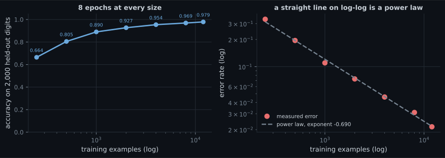
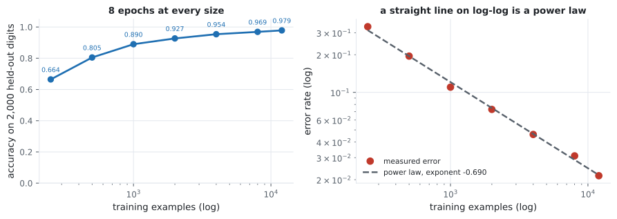
Examples	Accuracy	Error
250	0.6645	0.3355
1,000	0.8900	0.1100
4,000	0.9540	0.0460
12,000	0.9785	0.0215
~37,000 (extrapolated)	0.99	0.010
~101,000 (extrapolated)	0.995	0.005

Error falling as a power law in dataset size is one of the most reliable empirical facts in the field, and the exponent is usually shallow. Here it is −0.690: multiply the data by ten and the error falls by about a factor of five.

Treat the extrapolated rows as what they are — an extrapolation from seven points on one task, with the fit’s assumptions carried along. The shape is the point. Every additional nine of accuracy costs several times more data than the one before it, which is why the last few percent of a production model consumes most of the effort, and why “we’ll just collect more data” stops being a plan at some point.

Confidence is not uncertainty

Four separate experiments on this page produced the same finding, which is worth collecting:

Situation	Accuracy	Mean confidence
6-pixel shift	0.0265	0.7308
Inverted colours	0.1705	0.7940
Adversarial, ε = 0.2	0.3250	0.8035
Quarter contrast (works fine)	0.9610	0.6592

The last row is the sharpest. The model is less confident on the input it handles almost perfectly than on three inputs it gets catastrophically wrong. A softmax output is a normalised score, not a probability of being correct, and thresholding on it would reject good predictions while accepting nonsense.

diagram Diagram mermaid

  flowchart TD
  M["a 0.9785 model"] --> A["shift 4px"]
  M --> B["rotate 45 degrees"]
  M --> C["invert colours"]
  M --> D["adversarial noise"]
  M --> E["random noise"]
  A --> R1["0.0975"]
  B --> R2["0.4800"]
  C --> R3["0.1705"]
  D --> R4["0.3250"]
  E --> R5["0.9850 - unchanged"]
  R1 -.-> F["all still ~0.78 confident"]
  R3 -.-> F
  R4 -.-> F

sketch Accuracy against confidence, per failure p5.js

Click a transformation to see what it did to this model. The bars are the measured accuracy and the model's own confidence on the same inputs.

What is being done about it

Each measured limitation has an active research direction, and each is a partial answer rather than a solution:

Brittleness to transformation — data augmentation (measured on the augmentation page), and architectures with invariance built in rather than learned.
Adversarial examples — adversarial training, which raises robustness and costs clean accuracy. Nine years after they were described there is no defence that is both cheap and general.
Data hunger — self-supervised pretraining, which is the single biggest practical change since this module’s contents were standard: learn the representation from unlabelled data, then fine-tune on the few labels you have.
Miscalibration — temperature scaling, deep ensembles, and evidential methods. All improve on a raw softmax; none make it trustworthy out of the box.
No causal model — the deepest gap, and the one with the least engineering traction. A network that has never seen a rotated digit has no way to reason that rotation should not matter.

sketch The measured table, ranked p5.js

Click a column to rank every row by it. The bars are that column's values and the highest and lowest are computed from the numbers, not written in.

Pitfalls

Reading a benchmark number as a capability. 0.9785 on held-out MNIST became 0.0975 after a four-pixel shift.
Assuming convolution gives shift invariance. It gives equivariance; Flatten discards it.
Using softmax confidence as an uncertainty estimate. The model was less confident when right (0.6592) than when catastrophically wrong (0.7940).
Testing robustness with random noise. It left accuracy at 0.9850 while an equal-magnitude adversarial step reached 0.3250.
Extrapolating a power law far past the data. The 101,000-example figure is a projection from seven points, not a measurement.
Believing more data always fixes it. With exponent −0.690, each additional nine costs several times the previous total.
Evaluating only on the distribution you trained on. Every failure here is invisible to a standard test-set score.

Recap

A 0.9785 model fell to 0.0975 under a four-pixel shift and 0.4800 under a 45° rotation.
Convolution is translation-equivariant, not invariant — invariance comes from data or architecture.
Adversarial noise at ε = 0.2 gave 0.3250 while random noise of the same size gave 0.9850.
Error follows a power law with exponent −0.690; 99% would need roughly 37,000 examples against the 12,000 used.
Confidence stayed near 0.78 through every catastrophic failure and dropped to 0.6592 on an input handled correctly.
Each limitation has an active research direction and none has a complete answer.

That closes the scaling and deployment phase, and the taught material of this module: Phase 8 - Scaling & Deploying Deep Models collects what every page in it measured.

pch.quizTag pch.quizDefaultTitle

A convnet at 0.9785 accuracy fell to 0.0975 when test images were shifted four pixels. Why doesn't convolution prevent this?

pch.quizShowAnswer

B — Convolution is translation-EQUIVARIANT — the feature map shifts with the input — but the Flatten layer maps each spatial position to fixed dense weights, so a moved feature multiplies entirely different parameters — Pooling buys a little tolerance — one pixel still scored 0.9495 — but invariance has to come from training data or from an architecture designed for it.
At epsilon 0.2, adversarial noise gave 0.3250 accuracy while random noise of identical magnitude gave 0.9850. What does the comparison establish?

pch.quizShowAnswer

B — It is not noise-sensitivity at all — the model is untouched by random perturbation and destroyed by one specific direction, which means the decision boundary passes far closer to each point than its accuracy suggests — Without the random-noise control the result would be ambiguous. With it, the finding is about the geometry of the learned function.
The model scored 0.6592 mean confidence on quarter-contrast images it classified at 0.9610, and 0.7940 on inverted images it classified at 0.1705. What follows?

pch.quizShowAnswer

B — Softmax output is a normalised score, not a probability of being correct — thresholding on it would reject good predictions while accepting catastrophically wrong ones — Being less confident when right than when wrong is the clearest possible demonstration that the number is not an uncertainty estimate.
Error followed a power law with exponent -0.690 in dataset size. What does that imply for reaching 99.5% accuracy?

pch.quizShowAnswer

B — Roughly 101,000 examples against the 12,000 used — each additional nine of accuracy costs several times the data of the one before, which is why the last few percent dominates the effort — That figure is an extrapolation from seven measured points, so the shape of the curve is the finding rather than the precise number.
Which research direction most directly targets the data-hunger limitation?

pch.quizShowAnswer

B — Self-supervised pretraining — learn a representation from unlabelled data, then fine-tune on the few labels available — Adversarial training targets fragility and temperature scaling targets calibration; each limitation has its own partial answer rather than one fix.

🧪 Try It Yourself

pch.coffeeTagline

pch.coffeeCta

pch.feedbackHeading

pch.feedbackSubheading