Creating a Test Set (Avoiding Data Snooping)

What you’ll learn

what data snooping is, and why your own brain is the leak
how to split, and why random_staterandom_state alone is not a stable strategy
stratified sampling, and the exact distortion a random split introduces here
hash-based splitting that survives new rows arriving
the three situations where a random split is not merely suboptimal but wrong
how big a test set should be, with the arithmetic

Intuition

You are about to spend hours exploring this dataset. Every pattern you notice will influence the model you build — which features you engineer, which model family you try, which threshold looks reasonable. That is the point of exploration.

But if you explore all the data, those choices are informed by rows you will later use to measure success. The measurement is no longer independent, and the number it produces is optimistic by an amount you cannot estimate. There is no test to detect this and no correction for it afterwards.

The defence is procedural, not technical: split first, then explore only the training set. Set the test set aside now, before you know anything, and do not look at it again until the model is finished.

diagram Diagram mermaid

  flowchart LR
  A["Full dataset
20,640 districts"] --> B["Split immediately"]
  B --> C["Training set
16,512 rows"]
  B --> D["Test set
4,128 rows
locked away"]
  C --> E["Explore, engineer,
train, cross-validate"]
  E --> F["Final model"]
  F --> G["Evaluate once"]
  D --> G

The math: how big should the test set be?

The test estimate is itself a sample statistic, with a standard error. For an error rate $p$ measured on $n$ test rows:

\text{SE} = \sqrt{\frac{p(1-p)}{n}}

and the 95% interval is roughly $\pm 1.96\,\text{SE}$ . So:

Test rows	SE at $p = 0.1$	95% interval width
100	0.030	±5.9 points
1,000	0.009	±1.9 points
4,128	0.005	±0.9 points
10,000	0.003	±0.6 points

The usual 20% is a heuristic, not a law. What matters is the absolute count: 20% of 500 rows is 100 test rows and an interval of ±6 points, which cannot distinguish an 88% model from a 92% one. With 20,640 rows, 20% gives 4,128 and a comfortably tight interval.

Rule of thumb: aim for a test set large enough that the interval is narrower than the difference you care about detecting.

The straightforward split

basic_split.py

import pandas as pd
from sklearn.model_selection import train_test_split
 
URL = ("https://raw.githubusercontent.com/ageron/handson-ml2/master/"
       "datasets/housing/housing.csv")
housing = pd.read_csv(URL)
 
train_set, test_set = train_test_split(housing, test_size=0.2, random_state=42)
 
print(len(train_set), len(test_set))     # 16512 4128

basic_split.py

import pandas as pd
from sklearn.model_selection import train_test_split
 
URL = ("https://raw.githubusercontent.com/ageron/handson-ml2/master/"
       "datasets/housing/housing.csv")
housing = pd.read_csv(URL)
 
train_set, test_set = train_test_split(housing, test_size=0.2, random_state=42)
 
print(len(train_set), len(test_set))     # 16512 4128

random_state=42random_state=42 makes the split reproducible for this exact dataframe. Append one row and every subsequent row can move sides, so a model retrained on refreshed data may be evaluated on rows it previously trained on.

A split that survives new data

Hash each row’s stable identifier and assign it by hash value. A row’s side then depends only on its own identifier, never on the size or order of the dataset:

hash_split.py

from zlib import crc32
 
import numpy as np
import pandas as pd
 
 
def in_test_set(identifier, test_ratio):
    """Deterministic per-row membership: the same id always lands the same side."""
    return crc32(np.int64(identifier)) < test_ratio * 2**32
 
 
def split_by_id(data, test_ratio, id_column):
    ids = data[id_column]
    in_test = ids.apply(lambda i: in_test_set(i, test_ratio))
    return data.loc[~in_test], data.loc[in_test]
 
 
housing = pd.read_csv(URL)
# A genuinely stable id. Row position is NOT stable if rows are ever reordered.
housing["id"] = housing["longitude"] * 1000 + housing["latitude"]
 
train_set, test_set = split_by_id(housing, 0.2, "id")
print(len(train_set), len(test_set))     # 16322 4318

hash_split.py

from zlib import crc32
 
import numpy as np
import pandas as pd
 
 
def in_test_set(identifier, test_ratio):
    """Deterministic per-row membership: the same id always lands the same side."""
    return crc32(np.int64(identifier)) < test_ratio * 2**32
 
 
def split_by_id(data, test_ratio, id_column):
    ids = data[id_column]
    in_test = ids.apply(lambda i: in_test_set(i, test_ratio))
    return data.loc[~in_test], data.loc[in_test]
 
 
housing = pd.read_csv(URL)
# A genuinely stable id. Row position is NOT stable if rows are ever reordered.
housing["id"] = housing["longitude"] * 1000 + housing["latitude"]
 
train_set, test_set = split_by_id(housing, 0.2, "id")
print(len(train_set), len(test_set))     # 16322 4318

The counts are not exactly 80/20 because hashing distributes approximately, and that is fine. New districts join whichever side their own id dictates; existing districts never move.

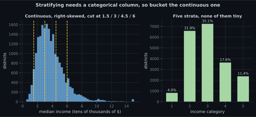
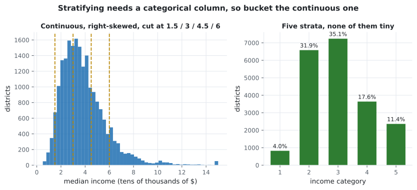
Stratified sampling

median_incomemedian_income is the strongest predictor of the target, so the test set must represent its distribution faithfully. A random split does not guarantee that.

Stratifying needs a categorical column, so bucket the continuous one first:

Left: histogram of median income with dashed cut lines at 1.5, 3.0, 4.5 and 6.0. Right: a bar chart of the resulting five categories with percentages from 4% to 35%. — The cut points are chosen so no stratum is tiny — the smallest holds 4% of districts. Too many buckets and each becomes too small to sample reliably.

stratified_split.py

import numpy as np
import pandas as pd
from sklearn.model_selection import StratifiedShuffleSplit, train_test_split
 
housing["income_cat"] = pd.cut(
    housing["median_income"],
    bins=[0.0, 1.5, 3.0, 4.5, 6.0, np.inf],
    labels=[1, 2, 3, 4, 5],
)
 
splitter = StratifiedShuffleSplit(n_splits=1, test_size=0.2, random_state=42)
train_idx, test_idx = next(splitter.split(housing, housing["income_cat"]))
strat_train = housing.iloc[train_idx]
strat_test = housing.iloc[test_idx]
 
overall = housing["income_cat"].value_counts(normalize=True).sort_index()
_, random_test = train_test_split(housing, test_size=0.2, random_state=42)
 
comparison = pd.DataFrame({
    "overall": overall,
    "stratified": strat_test["income_cat"].value_counts(normalize=True).sort_index(),
    "random": random_test["income_cat"].value_counts(normalize=True).sort_index(),
})
comparison["random % error"] = 100 * (comparison["random"] / comparison["overall"] - 1)
comparison["strat % error"] = 100 * (comparison["stratified"] / comparison["overall"] - 1)
print(comparison.round(4).to_string())
 
#             overall  stratified  random  random % error  strat % error
# income_cat
# 1            0.0398      0.0400  0.0402          0.9732         0.3650
# 2            0.3188      0.3188  0.3244          1.7323        -0.0152
# 3            0.3506      0.3505  0.3585          2.2664        -0.0138
# 4            0.1763      0.1764  0.1674         -5.0563         0.0275
# 5            0.1144      0.1143  0.1095         -4.3184        -0.0847
 
# Drop the helper column once the split is done
for subset in (strat_train, strat_test):
    subset.drop("income_cat", axis=1, inplace=True)

stratified_split.py

import numpy as np
import pandas as pd
from sklearn.model_selection import StratifiedShuffleSplit, train_test_split
 
housing["income_cat"] = pd.cut(
    housing["median_income"],
    bins=[0.0, 1.5, 3.0, 4.5, 6.0, np.inf],
    labels=[1, 2, 3, 4, 5],
)
 
splitter = StratifiedShuffleSplit(n_splits=1, test_size=0.2, random_state=42)
train_idx, test_idx = next(splitter.split(housing, housing["income_cat"]))
strat_train = housing.iloc[train_idx]
strat_test = housing.iloc[test_idx]
 
overall = housing["income_cat"].value_counts(normalize=True).sort_index()
_, random_test = train_test_split(housing, test_size=0.2, random_state=42)
 
comparison = pd.DataFrame({
    "overall": overall,
    "stratified": strat_test["income_cat"].value_counts(normalize=True).sort_index(),
    "random": random_test["income_cat"].value_counts(normalize=True).sort_index(),
})
comparison["random % error"] = 100 * (comparison["random"] / comparison["overall"] - 1)
comparison["strat % error"] = 100 * (comparison["stratified"] / comparison["overall"] - 1)
print(comparison.round(4).to_string())
 
#             overall  stratified  random  random % error  strat % error
# income_cat
# 1            0.0398      0.0400  0.0402          0.9732         0.3650
# 2            0.3188      0.3188  0.3244          1.7323        -0.0152
# 3            0.3506      0.3505  0.3585          2.2664        -0.0138
# 4            0.1763      0.1764  0.1674         -5.0563         0.0275
# 5            0.1144      0.1143  0.1095         -4.3184        -0.0847
 
# Drop the helper column once the split is done
for subset in (strat_train, strat_test):
    subset.drop("income_cat", axis=1, inplace=True)

Grouped bar chart of test-set proportion error by income category. Random-split bars reach plus 2.3 and minus 5.1 percent; stratified bars are near zero everywhere. — The random split under-represents category 4 by 5.1% and over-represents category 3 by 2.3%. The stratified split is within 0.4% everywhere, and within 0.1% for the four largest strata.

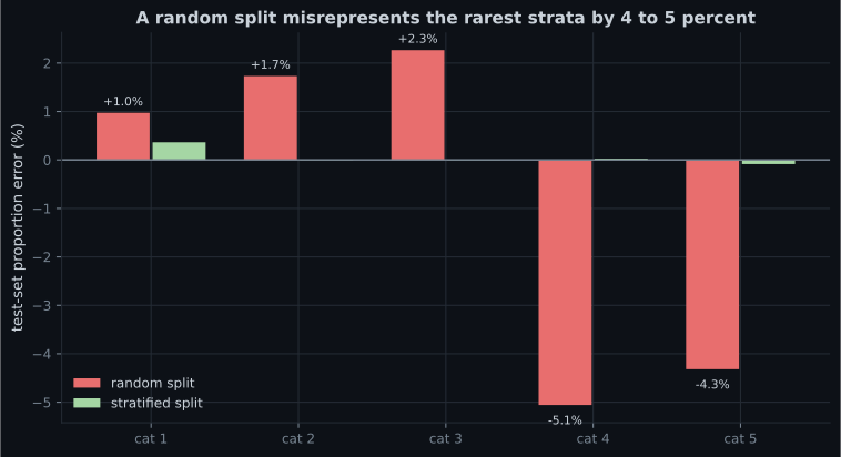
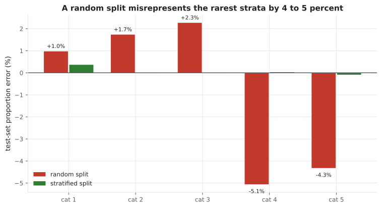
Reading the plot

The random split’s errors are not random noise you can average away — they are the specific composition of this test set, and every score you compute on it inherits them.
The error is worst for the middle-to-high strata. Category 4 is under-represented by 5%, so the test set contains proportionally fewer of exactly the districts the model is likely to find hardest.
Stratified is essentially exact. Errors below 0.1% for the four main strata. It costs one extra line.
Category 1 still shows 0.37% error even when stratified — with 4% of rows, integer rounding in the fold sizes leaves a residue. Rare strata are always approximate.

See it move

Two samplers drawing 20% from the same population, over and over. The bars show how far each sample’s stratum proportions drift from the population’s.

sketch Random versus stratified sampling p5.js

Both samplers draw 20% of the population repeatedly. The bars show the error in each stratum's proportion; the random sampler wanders, the stratified one stays pinned near zero.

When a random split is wrong

Stratification is a refinement. These three cases are different — a random split produces a number that is simply invalid:

Situation	What breaks	Correct split
Time series	Training on the future to predict the past	Split by date: train on older, test on newer
Grouped rows (several rows per patient, user, device)	The same entity appears on both sides	`GroupShuffleSplitGroupShuffleSplit` / `GroupKFoldGroupKFold` by entity
Spatial autocorrelation	Adjacent districts are near-duplicates	Split by region or block

The housing data has mild spatial autocorrelation — neighbouring districts resemble one another — so even the stratified split is slightly optimistic. For a production system you would split by county. This phase uses the random split because it is the version every tutorial uses, and the limitation is worth knowing rather than hiding.

Pitfalls

quizCheck yourself

Why must the test set be created before exploring the data?
Show answer
B — Because insights from the full dataset influence your modelling choices, so the test estimate stops being independent — and no correction exists afterwards — The leak runs through the analyst, not the code. A feature you invented after noticing a pattern in test rows was informed by those rows.
Why is random_state=42 not a sufficient strategy for a growing dataset?
Show answer
B — The split depends on the dataframe's contents, so adding rows can move existing rows between sets — and previously-tested rows end up in training — The permutation is over row positions. Hash-based splitting on a stable identifier fixes each row's side permanently, so new data can arrive safely.
In this dataset, how far does the random split misrepresent income category 4?
Show answer
C — By about 5% — The random test set contains 16.74% category-4 districts against 17.63% overall — a 5.06% relative shortfall. The stratified split is off by 0.03%.
You have one row per hospital visit and many visits per patient. What split do you need?
Show answer
B — A group split by patient, so no patient appears in both training and test — With a random split the model can memorise a patient from their training visits and be scored on their test visits. GroupShuffleSplit or GroupKFold keeps every patient on one side.

🧪 Try It Yourself

Exercise 1 – Split, and check the sizes

Exercise 2 – Bucket a continuous column

Exercise 3 – Measure the sampling bias

Exercise 4 – A split that survives new rows

Exercise 5 – How precise is a test estimate?

Recap

Split before exploring. The leak runs through your decisions, and no statistical correction exists for it.
Test-set precision follows $\sqrt{p(1-p)/n}$ ; 20% is a heuristic, and the absolute row count is what matters.
random_staterandom_state is reproducible only for a fixed dataframe. Hash a stable identifier when new data will arrive.
On this dataset a random split misrepresents income category 4 by 5.06%; stratified sampling brings the worst error to 0.36%.
Time series, grouped rows and spatial data need date, group and region splits respectively — a random split there is invalid, not merely imprecise.
Drop the stratification helper column once the split is made.

Exercise 6 – A split that survives new rows

Continue to Exploratory Data Analysis & Correlations — now that the test set is safely locked away, explore the training set as aggressively as you like.

If this helped you, consider buying me a coffee ☕

Buy me a coffee