
Data Cleaning & Handling Missing Values
What you’ll learn
Section titled “What you’ll learn”- MCAR, MAR and MNAR — the three mechanisms, and why only one is safe to ignore
- the three responses to a hole, and the arithmetic cost of each
- why every imputation understates variance, computed by hand
SimpleImputer, and why the imputer must be fitted on the training set only- the missing-indicator trick, which keeps the information that a value was absent
- a measured comparison of five strategies on real data
Intuition
Section titled “Intuition”A missing value is not nothing. It is a fact about the row that your model cannot read, and sometimes the most informative fact available — a blank income field on a loan application may predict default better than any number that could have been entered there.
So the question is never just “what number do I put here?” It is “why is this missing, and does the absence itself carry information?”
  flowchart TD
  A["Missing value found"] --> B{"Why is it missing?"}
  B -->|"pure chance"| C["MCAR
safe to impute or drop"]
  B -->|"depends on other columns"| D["MAR
impute using those columns"]
  B -->|"depends on the missing value itself"| E["MNAR
imputation biases the model"]
  C --> F["Add a missing-indicator anyway"]
  D --> F
  E --> G["Model the missingness explicitly"]
The three mechanisms
Section titled “The three mechanisms”| Mechanism | Definition | Example | Safe to impute? |
|---|---|---|---|
| MCAR | Missing completely at random | A sensor dropped packets at random | Yes |
| MAR | Missingness depends on other observed columns | Older records lack a field added later | Yes, using those columns |
| MNAR | Missingness depends on the missing value itself | High earners decline to state income | No — any imputation is biased |
MNAR is the dangerous one and it cannot be detected from the data alone: the evidence you would need is exactly what is absent. It has to be reasoned about from how the data was collected.
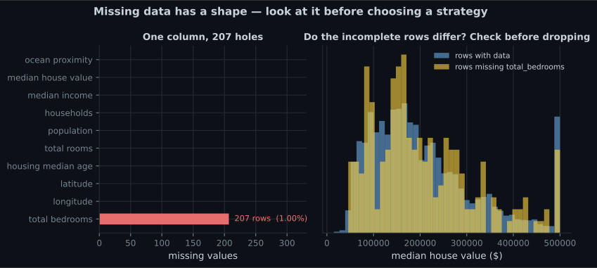
For total_bedrooms, 207 rows out of 20,640, the distribution of house values among incomplete
rows looks like the rest of the dataset — consistent with MCAR, and imputation is safe.
The three responses
Section titled “The three responses”# Option 1 — drop the rows with holes
housing.dropna(subset=["total_bedrooms"]) # loses 207 rows (1.0%)
# Option 2 — drop the whole column
housing.drop("total_bedrooms", axis=1) # loses a feature for all 20,640 rows
# Option 3 — fill the holes
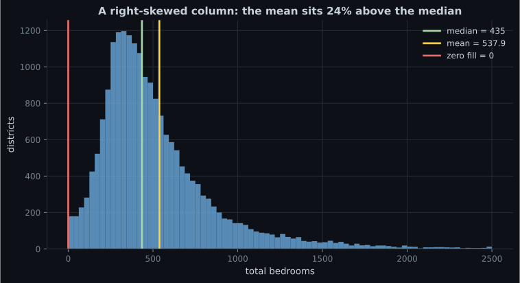
median = housing["total_bedrooms"].median() # 435.0
housing["total_bedrooms"].fillna(median, inplace=True)| Option | Cost | Choose it when |
|---|---|---|
| Drop rows | Loses whole observations | Very few rows affected, and MCAR |
| Drop column | Loses a feature entirely | Most of the column is missing (>40–50%) |
| Impute | Distorts the distribution | The default for everything else |
Option 3 wins here: losing 1% of rows to save one column is a bad trade, and losing the column across 100% of rows to save 1% is a worse one.
Worked example by hand: imputation shrinks variance
Section titled “Worked example by hand: imputation shrinks variance”Eight readings, two of them missing:
Step 1 — statistics of what is present. Six values, summing to 4,500:
The mean is more than double the median, because one reading of 3,000 drags it. This is the argument for median imputation in one line.
Step 2 — fill with the mean and recompute.
The mean is unchanged at 750 by construction. The standard deviation is not:
A 15% drop in spread, from adding no new information at all. Every imputed value sits exactly at the centre, contributing zero deviation, while still counting toward . Mean imputation always does this.
Step 3 — fill with the median instead. The mean shifts to 650 and becomes 957.30 — still contracted, but the centre is no longer distorted by the outlier.
| mean | std | |
|---|---|---|
| observed values only | 750.00 | 1111.31 |
| mean-imputed | 750.00 | 939.22 |
| median-imputed | 650.00 | 957.30 |
Both understate the spread. Any downstream statistic that depends on variance — a confidence interval, a t-test, a standardisation — is now slightly wrong, and the error grows with the fraction imputed. At 1% of one column, negligible. At 30%, serious.
See it move
Section titled “See it move”The hand-worked example used two missing values out of eight. The sketch scales that up: a skewed column of 400 rows where the missing fraction sweeps from 0% to 45%, filled with either the mean or the median. The histogram shows where the filled rows land, and the panel tracks the spread against the observed-only baseline.
Two behaviours to separate. Spread loss happens under both strategies and grows with the missing fraction — the green spike contributes zero deviation while still counting toward . Mean shift is strategy-specific: median fill keeps the centre where the observed data put it but moves the reported mean, while mean fill holds the mean fixed by construction. Neither is free, and at 45% missing neither is defensible — that is the point at which the honest move is to drop the column or model the missingness itself.
SimpleImputer
Section titled “SimpleImputer”fillna works, but it does not remember. SimpleImputer learns the fill values during fit and
replays them during transform, which is exactly what you need for a test set or a live request.
import pandas as pd
from sklearn.impute import SimpleImputer

housing_num = housing.select_dtypes("number")     # imputer needs numeric only

imputer = SimpleImputer(strategy="median")
imputer.fit(housing_num)

print(imputer.statistics_.round(2))
# one learned median per column, in column order

X = imputer.transform(housing_num)                # returns a NumPy array
housing_tr = pd.DataFrame(X, columns=housing_num.columns, index=housing_num.index)

print(housing_tr.isna().sum().sum())              # 0
Three details that matter:
- It learns a value for every numeric column, not just the one with holes. A column that has no missing values today may have them in production.
transformreturns a plain NumPy array. Wrap it back into a DataFrame if you want the column names.fitmust see the training data only. Compute the median over train and test together and test information has entered your training pipeline.
The estimator API
Section titled “The estimator API”SimpleImputer is the first place the scikit-learn object model becomes visible, and every
component in this phase follows it:
| Kind | Methods | Examples |
|---|---|---|
| Estimator | fit(X[, y]) — learns parameters | Every object here |
| Transformer | transform(X), fit_transform(X) | SimpleImputer, StandardScaler, OneHotEncoder |
| Predictor | predict(X), score(X, y) | LinearRegression, RandomForestClassifier |
Learned parameters end with an underscore (imputer.statistics_, scaler.mean_); constructor
arguments do not (strategy, n_estimators). That naming convention is how you tell what was
learned from what was chosen.
Keeping the information that a value was missing
Section titled “Keeping the information that a value was missing”If missingness carries signal, imputing destroys it. add_indicator=True keeps both:
from sklearn.impute import SimpleImputer

imputer = SimpleImputer(strategy="median", add_indicator=True)
X = imputer.fit_transform(housing_num)

print(housing_num.shape)     # (20640, 9)
print(X.shape)               # (20640, 10)  <- one extra binary column
The extra column is 1 wherever total_bedrooms was missing. Costs one column, and lets the model
decide for itself whether absence matters. Under MNAR it is not optional.
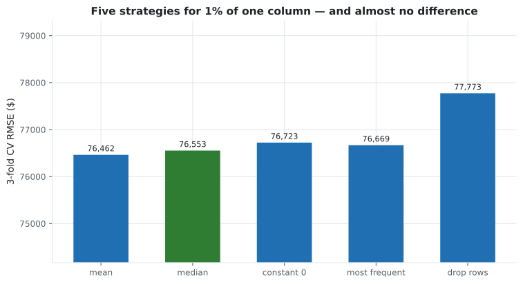
Does the strategy actually matter?
Section titled “Does the strategy actually matter?”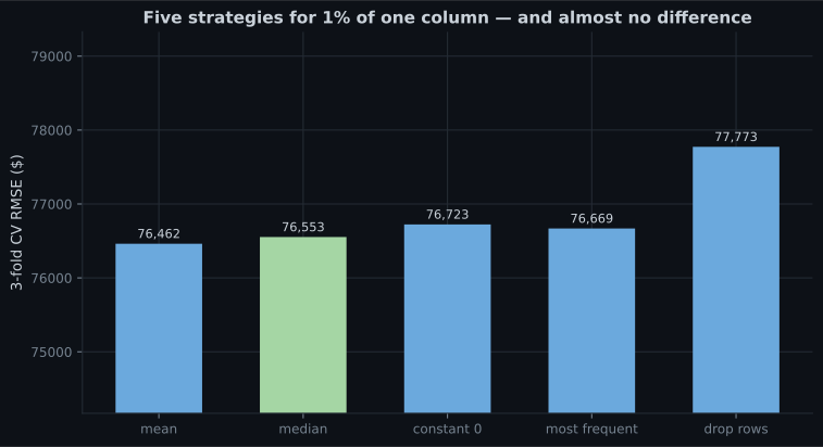
Reading the plot
Section titled “Reading the plot”- Every strategy is within noise of the others. With 1% of one column missing, the debate is not worth having on this dataset.
- Dropping rows scores comparably too, which is the MCAR check confirming itself: the removed rows were not special.
- Even constant-zero fill barely hurts, because a random forest can split around the artificial value.
- The scale changes the conclusion. At 30% missing, or if the mechanism were MNAR, these bars would separate sharply. The lesson is to measure rather than to assume the choice is free.
Pitfalls
Section titled “Pitfalls”-
High earners systematically decline to report their income. Which mechanism is that?
Missingness depends on the unobserved value itself, which is MNAR. Any imputation biases the column downward, and the bias cannot be detected from the data alone.
pch.quizShowAnswer
C — MNAR — Missingness depends on the unobserved value itself, which is MNAR. Any imputation biases the column downward, and the bias cannot be detected from the data alone.
-
You fill two of eight values with the column mean. What happens to the standard deviation?
In the worked example it drops from 1111.31 to 939.22 — a 15% contraction from adding no information. Every imputation understates variance.
pch.quizShowAnswer
B — It falls, because the imputed values sit exactly at the centre and contribute zero deviation while still counting toward n — In the worked example it drops from 1111.31 to 939.22 — a 15% contraction from adding no information. Every imputation understates variance.
-
Why fit SimpleImputer rather than just calling fillna with the median?
Recomputing the median on the test set means the test data influenced its own preprocessing. The fitted imputer replays the training values exactly.
pch.quizShowAnswer
B — The imputer stores the learned medians so the identical values can be reapplied to the test set and to live requests — Recomputing the median on the test set means the test data influenced its own preprocessing. The fitted imputer replays the training values exactly.
-
Five imputation strategies produce cross-validated RMSE within 1% of each other. What is the right conclusion?
The finding is specific to this missingness rate and mechanism. The transferable lesson is to measure rather than to assume, in either direction.
pch.quizShowAnswer
B — On this dataset — 1% of one column, apparently MCAR — the choice is not worth agonising over, but the same test on 30% missing data could look completely different — The finding is specific to this missingness rate and mechanism. The transferable lesson is to measure rather than to assume, in either direction.
🧪 Try It Yourself
Section titled “🧪 Try It Yourself”Exercise 1 – Watch imputation shrink the variance
Section titled “Exercise 1 – Watch imputation shrink the variance”Exercise 2 – Mean against median on skewed data
Section titled “Exercise 2 – Mean against median on skewed data”Exercise 3 – Fit and inspect a SimpleImputer
Section titled “Exercise 3 – Fit and inspect a SimpleImputer”Exercise 4 – Keep the missingness as a feature
Section titled “Exercise 4 – Keep the missingness as a feature”Exercise 5 – Check the MCAR assumption
Section titled “Exercise 5 – Check the MCAR assumption”- MCAR, MAR and MNAR are three different problems. Only MNAR cannot be fixed by imputation, and only reasoning about collection can identify it.
- Drop rows, drop the column, or impute — and dropping rows has no equivalent at serving time.
- Every imputation shrinks variance: the worked example falls from to after filling two of eight values.
total_bedroomshas a mean 23.6% above its median, so median imputation is the safer default.SimpleImputerlearns fill values duringfitand replays them; underscore-suffixed attributes are what was learned.add_indicator=Truepreserves the fact that a value was missing.- On this dataset five strategies score within 1% of each other. Measure rather than assume — in either direction.
Exercise 6 – How much spread does imputation remove?
Section titled “Exercise 6 – How much spread does imputation remove?”Continue to
Handling Text & Categorical Attributes
— the numeric columns are now clean, and ocean_proximity is still text.
pch.coffeeTagline
pch.coffeeCtapch.feedbackHeading
pch.feedbackSubheading