What you’ll learn

• the eight stages, and which of them are loops rather than steps
• bad data against bad algorithms, measured: 0.1142 either way
• underfitting and overfitting as one number — the train/test gap
• why one held-out set is not enough, and what the train-dev set diagnoses
• the No Free Lunch theorem, demonstrated on four datasets where the winner keeps moving

The lifecycle

  flowchart TD
  A["1. Define the problem
what decision does this feed?"] --> B["2. Collect data"]
  B --> C["3. Clean + preprocess"]
  C --> D["4. Engineer features"]
  D --> E["5. Train"]
  E --> F["6. Evaluate + validate"]
  F -->|"not good enough"| C
  F --> G["7. Deploy"]
  G --> H["8. Monitor"]
  H -->|"drift, or new data"| C
  H -->|"the metric was wrong"| A

Two of those arrows matter more than the boxes. Evaluation loops back to data, not to model selection — that is where the measurement below points. And monitoring loops back to problem definition, because the most common discovery in production is that you optimised the wrong thing.

Bad data or bad algorithm?

Every practitioner eventually asks: is my model underperforming because the algorithm is wrong, or because the data is bad? It is worth putting numbers on both.

Same 1,200-row dataset, four algorithms, three data conditions:

Three quantities fall out:

• Swapping the algorithm on clean data: 0.7892 → 0.9033, a spread of 0.1142.
• Flipping 15% of the labels, best model to best model: 0.9033 → 0.7892, a cost of 0.1142.
• Cutting the data 8×, best model to best model: 0.9033 → 0.8267, a cost of 0.0767.

figureTwo levers, the same sizematplotlib

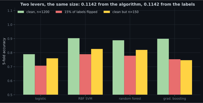
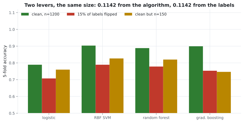
The popular slogan is “data beats algorithms”. The measurement says something more useful: the two levers are comparable in size, and you cannot substitute one for the other. The best algorithm on corrupted labels (0.7892) is no better than the worst algorithm on clean data (0.7892) — exactly equal, which is a coincidence, but an instructive one.

The practical consequence: if your model is underperforming, look at the data first — not because data always matters more, but because a data problem cannot be fixed by any algorithm, while an algorithm problem takes ten minutes to test.

Underfitting and overfitting

The two failure modes of stage 5, and one number distinguishes them: the gap between training and held-out performance.

figureMore capacity always helps the training setmatplotlib

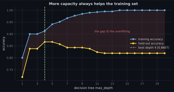
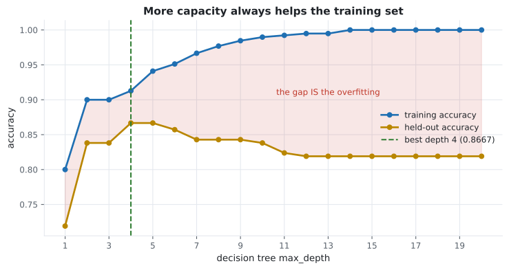
Underfitting is a low training score. The model is not flexible enough to capture the pattern even on data it has seen. Depth 1 above: 0.8000 on training.

Overfitting is a large gap. The model captured noise specific to the training rows. Depth 20: train 1.0000, held out 0.8190, gap 0.1810.

See it move

The pink curve is the point. It passes closer to every training point than the gold one does — its training error is genuinely lower — and it is wrong about the underlying shape. Watch it thrash while the gold curve, which describes the actual pattern, does not move at all.

Read the two numbers together and the diagnosis is immediate:

That last row is not a joke — it usually means the test set is easier than the training set, or the two have been swapped.

One held-out set is not enough

You split off a test set, tune your model, and report the test score. The problem: every tuning decision you made was informed by that test score, so it is no longer held out. You have leaked, a little, thirty times.

The standard fix is three splits: train, validation (tune here), and test (touch once). Phase 7 replaces the validation set with cross-validation, which is better still.

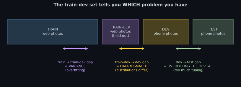
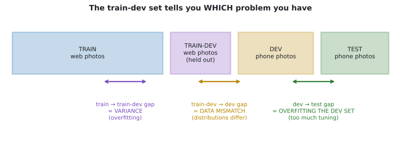
The train-dev set

There is a subtler failure the three-way split cannot diagnose. Suppose you train an image classifier on web photos, but production is phone photos. Your validation and test sets are phone photos — correctly, since that is what you will serve. Training score 0.98, validation score 0.83.

Is that overfitting, or is it that phone photos are simply different from web photos? The split cannot tell you, and the two problems have opposite fixes: overfitting wants regularisation, data mismatch wants different training data.

Andrew Ng’s train-dev set resolves it. Hold out a slice of the training distribution — web photos the model never trained on — and score that too:

figureThe train-dev set tells you WHICH problem you havematplotlib

This is worth internalising early. Most “the model does not work in production” reports are data mismatch, and most teams respond by regularising, which does nothing.

No Free Lunch

Wolpert’s theorem says that averaged over all possible problems, every algorithm performs identically. The practical version is weaker and far more useful: there is no algorithm that wins on every dataset, so you must try several.

Four models, four datasets:

figureBest model per row is boxed — the box never stays in one columnmatplotlib

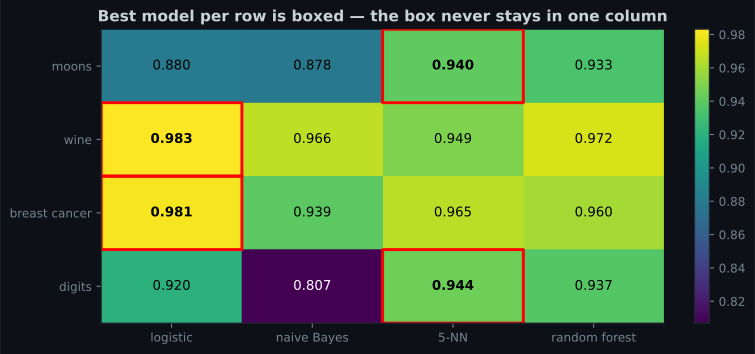
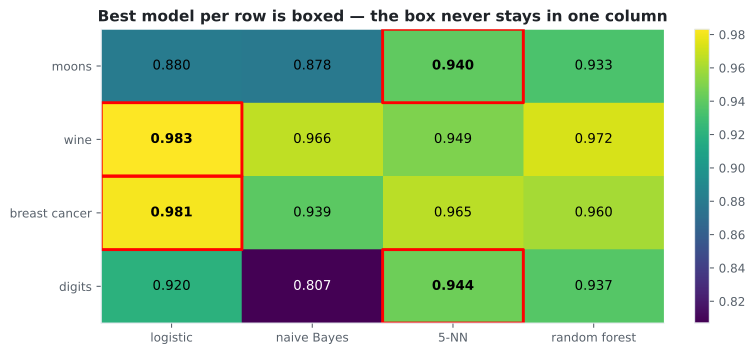
Note the practical implication for the lifecycle: stage 5 is not “choose the model”, it is “try four and measure”. That costs minutes.

Note also what the theorem does not say. It does not say all algorithms are equally good on your problem — they clearly are not, spanning 0.8069 to 0.9444 on digits. It says you cannot know which without checking.

Monitoring: the stage everyone skips

A deployed model has no idea the world has changed. The types page measured a batch model decaying from 0.9800 to 0.5100 under gentle drift, silently, with no error.

Three things worth monitoring, in increasing order of usefulness:

Input distributions. Cheap, immediate, no labels required. If the mean of a feature moves three standard deviations, something upstream changed.

Prediction distributions. Also label-free. If your fraud model suddenly flags 8% of transactions where it used to flag 2%, investigate before the metric arrives.

Actual performance. The only thing that really matters, and it requires labels, which usually arrive late — sometimes months late, for churn or default prediction. Build the label-collection pipeline on day one, not when the model starts failing.

In code

The evaluation half of the lifecycle, done properly:

from sklearn.datasets import make_classification
from sklearn.dummy import DummyClassifier
from sklearn.ensemble import HistGradientBoostingClassifier, RandomForestClassifier
from sklearn.linear_model import LogisticRegression
from sklearn.model_selection import cross_val_score, train_test_split
from sklearn.pipeline import make_pipeline
from sklearn.preprocessing import StandardScaler
from sklearn.svm import SVC
 
X, y = make_classification(n_samples=1200, n_features=20, n_informative=8,
                           n_redundant=4, class_sep=0.9, random_state=5)
 
# 1. Split off a test set FIRST and do not touch it again until the end.
X_dev, X_test, y_dev, y_test = train_test_split(
    X, y, test_size=0.2, random_state=0, stratify=y)
 
# 2. Baseline, so every later number is interpretable.
print("baseline", round(cross_val_score(DummyClassifier(), X_dev, y_dev, cv=5).mean(), 4))
 
# 3. Try several families — No Free Lunch says you cannot skip this.
candidates = {
    "logistic":      make_pipeline(StandardScaler(), LogisticRegression(max_iter=2000)),
    "RBF SVM":       make_pipeline(StandardScaler(), SVC()),
    "random forest": RandomForestClassifier(n_estimators=200, random_state=0),
    "boosting":      HistGradientBoostingClassifier(random_state=0),
}
scores = {n: cross_val_score(m, X_dev, y_dev, cv=5).mean() for n, m in candidates.items()}
for n, s in sorted(scores.items(), key=lambda kv: -kv[1]):
    print(f"  {n:15s} {s:.4f}")
 
# 4. ONE final number, on the untouched test set.
best_name = max(scores, key=scores.get)
final = candidates[best_name].fit(X_dev, y_dev).score(X_test, y_test)
print(f"chose {best_name}, test accuracy {final:.4f}")

from sklearn.datasets import make_classification
from sklearn.dummy import DummyClassifier
from sklearn.ensemble import HistGradientBoostingClassifier, RandomForestClassifier
from sklearn.linear_model import LogisticRegression
from sklearn.model_selection import cross_val_score, train_test_split
from sklearn.pipeline import make_pipeline
from sklearn.preprocessing import StandardScaler
from sklearn.svm import SVC
 
X, y = make_classification(n_samples=1200, n_features=20, n_informative=8,
                           n_redundant=4, class_sep=0.9, random_state=5)
 
# 1. Split off a test set FIRST and do not touch it again until the end.
X_dev, X_test, y_dev, y_test = train_test_split(
    X, y, test_size=0.2, random_state=0, stratify=y)
 
# 2. Baseline, so every later number is interpretable.
print("baseline", round(cross_val_score(DummyClassifier(), X_dev, y_dev, cv=5).mean(), 4))
 
# 3. Try several families — No Free Lunch says you cannot skip this.
candidates = {
    "logistic":      make_pipeline(StandardScaler(), LogisticRegression(max_iter=2000)),
    "RBF SVM":       make_pipeline(StandardScaler(), SVC()),
    "random forest": RandomForestClassifier(n_estimators=200, random_state=0),
    "boosting":      HistGradientBoostingClassifier(random_state=0),
}
scores = {n: cross_val_score(m, X_dev, y_dev, cv=5).mean() for n, m in candidates.items()}
for n, s in sorted(scores.items(), key=lambda kv: -kv[1]):
    print(f"  {n:15s} {s:.4f}")
 
# 4. ONE final number, on the untouched test set.
best_name = max(scores, key=scores.get)
final = candidates[best_name].fit(X_dev, y_dev).score(X_test, y_test)
print(f"chose {best_name}, test accuracy {final:.4f}")

Diagnosing the failure mode:

from sklearn.datasets import make_moons
from sklearn.model_selection import train_test_split
from sklearn.tree import DecisionTreeClassifier
 
X, y = make_moons(n_samples=600, noise=0.32, random_state=0)
X_tr, X_te, y_tr, y_te = train_test_split(X, y, test_size=0.35,
                                          random_state=0, stratify=y)
 
for depth in (1, 4, 20):
    m = DecisionTreeClassifier(max_depth=depth, random_state=0).fit(X_tr, y_tr)
    train, test = m.score(X_tr, y_tr), m.score(X_te, y_te)
    gap = train - test
    if train < 0.85:
        verdict = "UNDERFIT — not enough capacity"
    elif gap > 0.10:
        verdict = "OVERFIT — memorising the training rows"
    else:
        verdict = "reasonable"
    print(f"depth {depth:2d}: train {train:.4f}  test {test:.4f}  gap {gap:.4f}  {verdict}")
 
# depth  1: train 0.8000  test 0.7190  gap 0.0810  UNDERFIT — not enough capacity
# depth  4: train 0.9128  test 0.8667  gap 0.0462  reasonable
# depth 20: train 1.0000  test 0.8190  gap 0.1810  OVERFIT — memorising the training rows

from sklearn.datasets import make_moons
from sklearn.model_selection import train_test_split
from sklearn.tree import DecisionTreeClassifier
 
X, y = make_moons(n_samples=600, noise=0.32, random_state=0)
X_tr, X_te, y_tr, y_te = train_test_split(X, y, test_size=0.35,
                                          random_state=0, stratify=y)
 
for depth in (1, 4, 20):
    m = DecisionTreeClassifier(max_depth=depth, random_state=0).fit(X_tr, y_tr)
    train, test = m.score(X_tr, y_tr), m.score(X_te, y_te)
    gap = train - test
    if train < 0.85:
        verdict = "UNDERFIT — not enough capacity"
    elif gap > 0.10:
        verdict = "OVERFIT — memorising the training rows"
    else:
        verdict = "reasonable"
    print(f"depth {depth:2d}: train {train:.4f}  test {test:.4f}  gap {gap:.4f}  {verdict}")
 
# depth  1: train 0.8000  test 0.7190  gap 0.0810  UNDERFIT — not enough capacity
# depth  4: train 0.9128  test 0.8667  gap 0.0462  reasonable
# depth 20: train 1.0000  test 0.8190  gap 0.1810  OVERFIT — memorising the training rows

Pitfalls

Treating the lifecycle as linear. It has two loops. Evaluation sends you back to the data far more often than to the model.

Tuning on the test set. Thirty decisions informed by one number is thirty small leaks. Use a validation set or cross-validation, and touch the test set once.

Regularising when the real problem is data mismatch. The train-dev set exists exactly to distinguish these. Regularisation cannot fix training on web photos and serving phone photos.

Picking an algorithm before measuring. The winner moved between columns on all four datasets above. Trying four families costs minutes.

Judging on training accuracy. It reached 1.0000 at depth 20 while held-out accuracy was at its worst.

Shipping without monitoring. The measured decay is 0.9800 → 0.5100 with no alert. If you cannot detect that, you will find out from a user.

Defining the problem after building the model. Stage 1 exists because it is the cheapest stage to redo and the most expensive to get wrong.

Recap

• Eight stages, two loops: evaluation returns to the data, monitoring returns to the problem definition.
• The two levers are the same size: algorithm spread 0.1142, label-noise cost 0.1142, and 8× less data cost 0.0767.
• Underfitting is a low train score; overfitting is a large train/test gap. At depth 20: 1.0000 and 0.8190, gap 0.1810.
• One held-out set is not enough. Train / validation / test, and touch the test set once.
• The train-dev set separates variance from data mismatch — two problems with opposite fixes.
• No Free Lunch: the best model moved between columns on all four datasets.
• Monitoring is stage 8 and gets skipped, which is why silent decay is the most common production failure.

🧪 Try It Yourself

Exercise 1 – Split first, baseline first

Exercise 2 – Diagnose the failure mode

Exercise 3 – Bad labels beat every algorithm

Exercise 4 – No Free Lunch, demonstrated

Exercise 5 – Simulate the train-dev diagnosis

Exercise 6 – Price the act of choosing a model

Next

Setting up the ML Environment — the last practical step before Phase 2: a reproducible Python environment, pinned versions, and a sanity-check script.