
t-SNE and Manifold Learning
What you’ll learn
Section titled “What you’ll learn”- the manifold hypothesis, and why linear projection cannot exploit it
- the t-SNE objective: Gaussian similarities in, Student-t similarities out, KL divergence between
- what perplexity actually controls, measured by the KL divergence it reaches
- the two things t-SNE plots do not preserve — cluster size and cluster distance — quantified
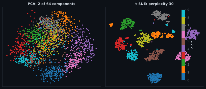
- trustworthiness as a number you can put on an embedding: PCA 0.830, t-SNE 0.992
- LLE and modified LLE, which unroll a Swiss roll that PCA merely flattens
- why t-SNE has no
transform, and what UMAP changes
Intuition
Section titled “Intuition”A grayscale image lives in 784 dimensions. But the set of images that look like handwritten digits is a vanishingly small part of that space — almost every point in is static. The digits occupy a thin, curved, low-dimensional sheet inside it.
That is the manifold hypothesis: real high-dimensional data concentrates near a low-dimensional manifold. If you could find the manifold’s own coordinates, you could describe each image with a handful of numbers instead of 784.
PCA assumes that manifold is flat. When it is not, PCA does the only thing a rotation can do: it photographs the curved surface from the best available angle, and everything on the far side lands on top of everything on the near side.
Manifold learning drops the flatness assumption. The methods differ in what they preserve instead:
- LLE preserves each point’s local linear relationship with its neighbours.
- Isomap preserves geodesic distances measured along the manifold.
- t-SNE preserves neighbourhood membership, and explicitly gives up on everything else.
  flowchart TD
  D["High-dimensional data"] --> Q{"Does it lie near a FLAT subspace?"}
  Q -->|"yes"| P["PCA — fast, invertible, preserves global structure"]
  Q -->|"no, it is curved"| M["Manifold learning"]
  M --> L["LLE / Isomap
reconstruct the manifold's coordinates"]
  M --> T["t-SNE / UMAP
preserve neighbourhoods for VISUALISATION"]
  T --> W["Global distances are NOT meaningful"]
The Swiss roll
Section titled “The Swiss roll”The standard demonstration is a 2-D sheet rolled up in 3-D. It is genuinely two-dimensional — every point has a position along the roll and a position across it — but the rolling makes points that are far apart along the sheet end up close together in space.
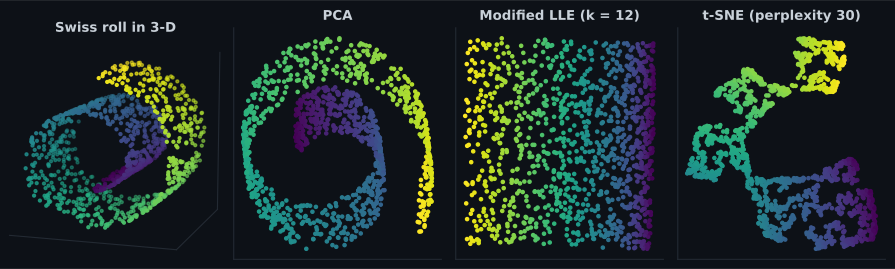
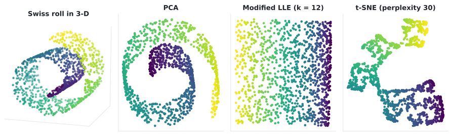
| Method | Trustworthiness () | What it produced |
|---|---|---|
| PCA | 0.9693 | The spiral, seen edge-on |
| LLE | 0.9953 | Unrolled, with some pinching |
| Modified LLE | 0.9942 | A clean rectangle |
| t-SNE | 0.9995 | Correct locally, torn globally |
Trustworthiness (defined below) measures whether points that are neighbours in the embedding were also neighbours in the original space. Every method scores well because that is a local question — and it is precisely the question t-SNE optimises.
The math
Section titled “The math”t-SNE builds two probability distributions over pairs of points and makes them match.
In the high-dimensional space, define a conditional probability that would pick as its neighbour, using a Gaussian centred on :
Each point gets its own bandwidth , which is what lets t-SNE handle regions of different density. Symmetrise:
In the low-dimensional space, use a Student-t distribution with one degree of freedom — a Cauchy — instead of a Gaussian:
Minimise the Kullback-Leibler divergence between them by gradient descent on the :
Why the heavy tail
Section titled “Why the heavy tail”That Student-t in the output is the “t” in t-SNE, and it exists to solve the crowding problem.
In dimensions you can place many more points at mutually moderate distances than you can in 2. The volume of a ball of radius grows like , so a neighbourhood that comfortably holds 1,000 points in 50-D has nowhere to put them in 2-D. If both distributions were Gaussian, the only way to fit everyone in would be to crush all the moderately-distant pairs into the centre.
The Cauchy’s heavy tail means a large output distance still produces a non-negligible . So a moderately-dissimilar pair can be placed far apart without incurring a big penalty, which frees up room in the middle for the genuinely-near pairs. Distant clusters get pushed apart and gaps open up.
Why KL divergence is asymmetric — and what that costs
Section titled “Why KL divergence is asymmetric — and what that costs”is weighted by . Look at the two error modes:
- Large , small (near in high-D, far in the map): the term is large. Heavily penalised.
- Small , large (far in high-D, near in the map): is tiny, so the whole term is tiny. Barely penalised.
t-SNE therefore works hard to keep neighbours together and hardly cares about keeping non-neighbours apart. Local structure is faithful; global structure is not constrained at all. That single asymmetry explains every caveat on this page.
Perplexity
Section titled “Perplexity”The bandwidth is not set directly. Instead you set a target perplexity, and t-SNE binary-searches each until the conditional distribution has that perplexity:
Perplexity is a smooth measure of “how many neighbours does this point effectively have?” A perplexity of 30 means each point’s Gaussian is widened or narrowed until it spreads its probability over roughly 30 others.
Perplexity, measured
Section titled “Perplexity, measured”On 800 digit images:
| Perplexity | Final KL divergence |
|---|---|
| 2 | 0.6316 |
| 5 | 0.6192 |
| 30 | 0.5016 |
| 100 | 0.4456 |
The KL divergence falls monotonically with perplexity — which is exactly why you must not choose perplexity by minimising KL. A larger perplexity spreads each over more points, making it a smoother target that a 2-D layout can match more easily. The objective is not comparable across perplexities.
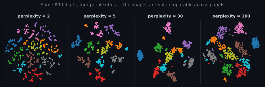
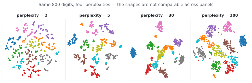
Practical guidance:
- The usual range is 5 to 50; 30 is the default and a good first try.
- Perplexity must be less than ; scikit-learn requires
perplexity < n_samples. - Run several and look for structure that survives. A cluster that appears at perplexity 5, 30 and 50 is probably real. One that appears only at perplexity 2 is probably not.
What the plot does not tell you
Section titled “What the plot does not tell you”This is the most important section on the page.
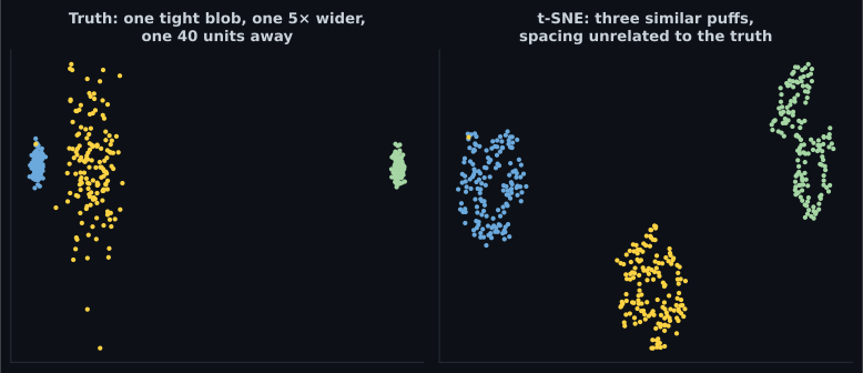
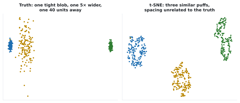
Take three groups whose true geometry is known: a tight blob at the origin, a blob five times wider centred 6 units away, and another tight blob 40 units away. Run t-SNE at perplexity 30 and measure what came out:
| Tight blob | Wide blob | Distant blob | |
|---|---|---|---|
| True mean radius | 0.383 | 1.941 | 0.345 |
| t-SNE mean radius | 5.562 | 5.805 | 6.245 |
A 5.6-fold difference in true size became a 1.1-fold difference in the plot. And the distances:
| Pair | True centre distance | t-SNE centre distance |
|---|---|---|
| tight ↔ wide | 6.04 | 38.35 |
| wide ↔ distant | 34.01 | 39.48 |
Two gaps differing by more than five-fold were rendered essentially identical.
Three rules follow, and they are not negotiable:
- Cluster sizes in a t-SNE plot are meaningless. Per-point bandwidths deliberately equalise density, so a sparse cluster and a dense one come out the same size.
- Distances between clusters are meaningless. The KL asymmetry barely penalises far-in-high-D pairs, so their spacing is essentially unconstrained.
- Apparent clusters may not be real. At low perplexity t-SNE produces crisp-looking clumps in uniform noise. Always check across perplexities.
What a t-SNE plot does tell you, reliably: which points are near which other points.
Trustworthiness: a number instead of a vibe
Section titled “Trustworthiness: a number instead of a vibe”sklearn.manifold.trustworthiness asks whether the nearest neighbours in the embedding were
also near in the original space:
where are the points in ‘s embedded neighbourhood that were not in its original neighbourhood, and is ‘s rank by distance from in the original space. It runs from 0 to 1, and it penalises false neighbours — pairs the map claims are close that were not.
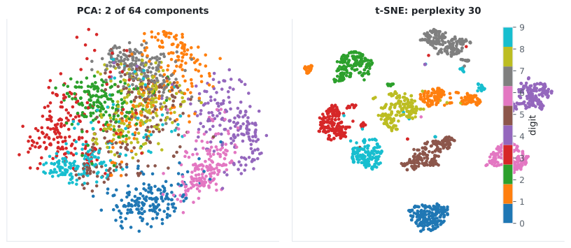
On the full digits dataset:
| Representation | Trustworthiness () | 5-NN accuracy (5-fold) |
|---|---|---|
| Raw 64-D | — | 0.9627 |
| PCA to 2-D | 0.8296 | 0.6032 |
| t-SNE to 2-D | 0.9917 | 0.9761 |
Two dimensions of t-SNE classify digits better than the original 64 dimensions. That is not because t-SNE created information — it is the curse of dimensionality working in reverse: nearest neighbours are more meaningful in 2-D when the 2-D layout was built specifically to preserve neighbourhoods.
Do not conclude that t-SNE is a good preprocessing step for classification. That 0.9761 was
computed on an embedding fitted to all the data, including the held-out folds. t-SNE has no
transform method, so you cannot embed a test set without refitting — which is exactly why this
number is a diagnostic, not a pipeline.
See it move
Section titled “See it move”The next sketch is the crowding problem itself — the reason for the Student-t tail.
At a Gaussian gives and the Student-t gives — over five hundred thousand times more. That difference is the space t-SNE uses to separate clusters instead of piling them on top of each other.
In code
Section titled “In code”from sklearn.datasets import load_digits
from sklearn.manifold import TSNE, trustworthiness
X, y = load_digits(return_X_y=True)
ts = TSNE(
n_components=2, # 2 or 3; anything higher is not what the method is for
perplexity=30, # effective neighbourhood size; try 5, 30, 50
init="pca", # far more stable than "random"; the default since 1.2
learning_rate="auto", # max(n / early_exaggeration / 4, 50)
random_state=0,
)
Z = ts.fit_transform(X)
print("KL divergence ", round(ts.kl_divergence_, 4))
print("iterations ", ts.n_iter_)
print("trustworthiness", round(trustworthiness(X, Z, n_neighbors=12), 4)) # 0.9917Note fit_transform — there is no fit followed by transform on new data. t-SNE optimises the
positions of these points; a new point has no defined position without rerunning the whole
optimisation.
Three parameters worth knowing:
init="pca" starts the optimisation from the PCA projection. It is more reproducible than
random initialisation and preserves a little global structure, which is close to free.
early_exaggeration (default 12) multiplies all during the first 250 iterations,
which forms tight clusters with wide gaps before the fine layout begins. Raise it if clusters are
not separating.
learning_rate — the classic default of 200 is too low for large and produces a
compressed “ball” with everything crushed together. "auto" scales it with and is what you
should use.
Preprocess with PCA first
Section titled “Preprocess with PCA first”For data with hundreds of features, reduce to about 50 with PCA before t-SNE. This is the standard recipe and it does three things: cuts the distance computation, suppresses noise dimensions, and usually improves the embedding.
from sklearn.decomposition import PCA
from sklearn.manifold import TSNE
from sklearn.pipeline import make_pipeline

# The standard recipe for wide data.
embed = make_pipeline(
    PCA(n_components=50, random_state=0),
    TSNE(n_components=2, perplexity=30, init="pca", random_state=0),
)
Z = embed.fit_transform(X)      # fit_transform only — there is no transform
Locally Linear Embedding
Section titled “Locally Linear Embedding”LLE takes a different route with no probabilities at all:
- For each point, find its nearest neighbours.
- Solve for the weights that best reconstruct as a linear combination of those neighbours, subject to .
- Find low-dimensional that are reconstructed by the same weights.
Step 2 captures the local geometry, and because the weights are constrained to sum to 1 they are invariant to rotation, rescaling and translation. Step 3 then asks: what layout in 2-D has the same local geometry?
from sklearn.datasets import make_swiss_roll
from sklearn.manifold import LocallyLinearEmbedding, trustworthiness

X, t = make_swiss_roll(n_samples=1200, noise=0.05, random_state=42)

std = LocallyLinearEmbedding(n_neighbors=12, n_components=2, random_state=0)
mod = LocallyLinearEmbedding(n_neighbors=12, n_components=2,
                             method="modified", random_state=0)

for name, model in (("standard", std), ("modified", mod)):
    Z = model.fit_transform(X)
    print(f"{name:9s} reconstruction_error_ {model.reconstruction_error_:.3e}"
          f"  trustworthiness {trustworthiness(X, Z, n_neighbors=12):.4f}")

# standard  reconstruction_error_ 1.073e-07  trustworthiness 0.9953
# modified  reconstruction_error_ 2.098e-06  trustworthiness 0.9942
Both score well on trustworthiness, but they look very different: standard LLE pinches the
rectangle at one end, while modified LLE (which uses several weight vectors per neighbourhood)
produces the clean rectangle in the figure above. Unlike t-SNE, LLE does have a transform
method — the weights generalise.
UMAP is the modern alternative. It optimises a similar neighbourhood-preservation objective from a topological rather than probabilistic derivation, and in practice:
- It is much faster — near-linear in against t-SNE’s with a larger constant.
- It preserves more global structure, so inter-cluster distances mean somewhat more (though still not enough to quantify).
- It has a
transformmethod, so it can be used in a pipeline.
It is not in scikit-learn (pip install umap-learn) and its n_neighbors plays the role of
perplexity. Its plots share the same caveats as t-SNE’s, just less severely.
pch.algoApi sklearn.manifold.TSNE
pch.algoAssumes
- Data lies near a lower-dimensional manifold
- Local neighbourhoods are what you care about
- You want a picture, not features for a downstream model
pch.algoCost
- pch.algoTrain
O(n log n) with the Barnes-Hut approximation (the default for n_components < 4)- pch.algoPredict
not supported at all — no transform method exists- pch.algoMemory
O(n log n) with Barnes-Hut; O(n^2) with the exact method
p_ij — high-dimensional pair similarity; q_ij — low-dimensional pair similarity; Perp — 2 to the power of the Shannon entropy of P_i
pch.algoHyperparams
-
perplexitydefault 30 Effective neighbourhood size. Try 5, 30 and 50; keep the structure that appears in all three. -
initdefault 'pca' PCA initialisation is more reproducible than random and retains a little global structure. -
learning_ratedefault 'auto' The old default of 200 crushes large datasets into a ball. Leave it on auto. -
early_exaggerationdefault 12.0 Inflates p_ij for the first 250 iterations to open gaps between clusters. -
n_iterdefault 1000 Rarely needs raising. Check kl_divergence_ has stopped falling. -
metricdefault 'euclidean' Use 'cosine' for text embeddings, or 'precomputed' with your own distance matrix.
pch.algoReachFor
- You want to see whether high-dimensional data has cluster structure
- You are exploring embeddings from a neural network or a language model
- You need a figure for a paper or a stakeholder
- n is under about 100,000
pch.algoLookElsewhere
- You need features for a downstream model — there is no transform, so it cannot go in a pipeline
- You need distances or cluster sizes in the output to be meaningful — they are not
- You need reproducibility across data updates — adding one row changes the whole layout
- n is in the millions — use UMAP
Pitfalls
Section titled “Pitfalls”Measuring anything off the plot. Cluster radii were equalised from a 5.6× ratio to 1.1×, and gaps of 6.04 and 34.01 both came out near 39. Neither size nor distance survives.
Choosing perplexity by minimising KL divergence. It falls monotonically with perplexity — 0.6316 at 2, 0.4456 at 100 — because larger perplexity is an easier target. It is not a model selection criterion.
Believing clusters that appear at one perplexity. Low perplexity manufactures crisp clumps out of noise. Run 5, 30 and 50 and keep only what persists.
Trying to use it in a pipeline. TSNE has fit_transform and no transform. Any
cross-validation score computed on a t-SNE embedding of the full dataset — including the 0.9761
quoted above — has seen the held-out folds.
Leaving learning_rate=200 on large data. On tens of thousands of points this produces a
single dense ball. "auto" is the fix.
Running it on raw high-dimensional data. Reduce to about 50 dimensions with PCA first. Faster, less noisy, usually a better result.
Comparing two t-SNE runs. Different seeds give different layouts of the same structure. Two plots are not comparable point-by-point; only the neighbourhood structure is.
Treating it as an alternative to PCA. They do different jobs. PCA is a reusable, invertible transform that preserves global geometry. t-SNE is a one-shot picture that preserves neighbourhoods.
Compare
Section titled “Compare”| PCA | t-SNE | UMAP | LLE | Isomap | |
|---|---|---|---|---|---|
| Linear | yes | no | no | no | no |
Has transform | yes | no | yes | yes | yes |
| Invertible | yes | no | no | no | no |
| Preserves global distance | yes | no | partly | no | yes (geodesic) |
| Preserves local neighbours | poorly | best | very well | well | well |
| Digits trustworthiness | 0.830 | 0.992 | ~0.99 | — | — |
| Speed | fastest | slow | fast | moderate | slow |
| Main parameter | n_components | perplexity | n_neighbors | n_neighbors | n_neighbors |
-
In a t-SNE plot, cluster A looks twice as wide as cluster B. What can you conclude?
Measured on this page: true radii of 0.383, 1.941 and 0.345 — a 5.6-fold spread — came out as 5.56, 5.81 and 6.25. Each point gets its own sigma_i chosen to hit the target perplexity, which deliberately normalises away density differences.
pch.quizShowAnswer
B — Nothing — per-point bandwidths equalise density, so relative cluster sizes are not preserved — Measured on this page: true radii of 0.383, 1.941 and 0.345 — a 5.6-fold spread — came out as 5.56, 5.81 and 6.25. Each point gets its own sigma_i chosen to hit the target perplexity, which deliberately normalises away density differences.
-
Why does t-SNE use a Student-t distribution in the output space rather than a Gaussian?
In 2-D there is far less room than in 50-D for points at moderate distances. With a Gaussian, everything would be crushed into the middle. At output distance 4 the Student-t gives 0.0588 where a Gaussian gives 1.1e-7 — that gap is the room t-SNE uses to separate clusters.
pch.quizShowAnswer
B — Its heavy tail lets moderately-distant pairs sit far apart cheaply, solving the crowding problem — In 2-D there is far less room than in 50-D for points at moderate distances. With a Gaussian, everything would be crushed into the middle. At output distance 4 the Student-t gives 0.0588 where a Gaussian gives 1.1e-7 — that gap is the room t-SNE uses to separate clusters.
-
Your t-SNE run at perplexity 100 has a lower KL divergence than at perplexity 5. Which is better?
Measured: 0.6316 at perplexity 2 down to 0.4456 at 100. Larger perplexity spreads each P_i over more points, making a smoother distribution that a 2-D layout matches more easily. Choose perplexity by running several and keeping the structure that persists.
pch.quizShowAnswer
B — You cannot tell — KL falls monotonically with perplexity because larger perplexity is an easier target — Measured: 0.6316 at perplexity 2 down to 0.4456 at 100. Larger perplexity spreads each P_i over more points, making a smoother distribution that a 2-D layout matches more easily. Choose perplexity by running several and keeping the structure that persists.
-
Why does TSNE have no transform method?
There is no learned mapping — only n optimised 2-D positions. That is also why any cross-validation score computed on a t-SNE embedding of the whole dataset, including the 0.9761 on this page, has leaked the held-out folds.
pch.quizShowAnswer
B — The embedding coordinates are free parameters optimised for these specific points; a new point has no defined position without rerunning the optimisation — There is no learned mapping — only n optimised 2-D positions. That is also why any cross-validation score computed on a t-SNE embedding of the whole dataset, including the 0.9761 on this page, has leaked the held-out folds.
-
PCA gives 0.830 trustworthiness on the digits and t-SNE gives 0.992. What does that measure?
Trustworthiness penalises FALSE neighbours — pairs the map draws close together that were far apart originally. It measures exactly what t-SNE optimises, which is why t-SNE wins so decisively and why the score says nothing about global structure.
pch.quizShowAnswer
B — Whether points that are neighbours in the 2-D map were also neighbours in the original 64-D space — Trustworthiness penalises FALSE neighbours — pairs the map draws close together that were far apart originally. It measures exactly what t-SNE optimises, which is why t-SNE wins so decisively and why the score says nothing about global structure.
🧪 Try It Yourself
Section titled “🧪 Try It Yourself”Exercise 1 – PCA cannot unroll a Swiss roll
Section titled “Exercise 1 – PCA cannot unroll a Swiss roll”Exercise 2 – The perplexity sweep
Section titled “Exercise 2 – The perplexity sweep”Exercise 3 – Measure what the plot destroys
Section titled “Exercise 3 – Measure what the plot destroys”Exercise 4 – Distances between clusters are erased too
Section titled “Exercise 4 – Distances between clusters are erased too”Exercise 5 – Trustworthiness against neighbour accuracy
Section titled “Exercise 5 – Trustworthiness against neighbour accuracy”- The manifold hypothesis: real high-dimensional data lies near a low-dimensional surface. PCA assumes that surface is flat; manifold learning does not.
- t-SNE matches Gaussian similarities in high-D against Student-t similarities in 2-D by minimising KL divergence. The heavy tail solves the crowding problem — at distance 4 it is over 500,000 times larger than a Gaussian.
- The KL asymmetry penalises splitting up neighbours heavily and barely penalises putting non-neighbours together, so local structure is faithful and global structure is not.
- Cluster sizes are meaningless: radii of 0.383, 1.941 and 0.345 all came out near 6.
- Cluster distances are meaningless: gaps of 6.04 and 34.01 both came out near 39.
- Perplexity is the effective neighbourhood size. KL falls monotonically with it (0.6316 → 0.4456), so it cannot be tuned that way — run several and keep what persists.
- Trustworthiness quantifies neighbourhood preservation: PCA 0.830, t-SNE 0.992 on digits.
- t-SNE has no
transform. LLE and UMAP do.
Exercise 6 – Check whether the distances survived
Section titled “Exercise 6 – Check whether the distances survived”That completes Phase 6. Go back to the
phase overview
for the practice project, or move on to
Phase 7 - Model Optimization & Tuning,
where every one of these choices — , eps, perplexity, the number of components — becomes
something you select with cross-validation rather than by eye.
pch.coffeeTagline
pch.coffeeCtapch.feedbackHeading
pch.feedbackSubheading