What you’ll learn

• the three drift types, stated precisely enough to tell apart
• the measurement that matters: input monitoring is neither necessary nor sufficient
• PSI and the KS statistic, with the shift each one needs before it notices
• why a label lag makes your accuracy dashboard a picture of the past
• what to actually monitor, in what order, and what to do when it fires

Three kinds of drift

The vocabulary gets used loosely, which is why teams end up applying the wrong fix. Stated as distributions, the distinction is exact.

Your model learned to approximate $P(y \mid X)$ from a training sample of $P(X)$. Two things can change independently:

Covariate drift (also data drift): $P(X)$ changes, $P(y \mid X)$ does not. Your users get younger, a sensor recalibrates, a new marketing channel brings different traffic. The relationship you learned is still true — you are just seeing different inputs.

Concept drift: $P(y \mid X)$ changes. The relationship itself moved. Fraud tactics evolve, a competitor changes prices, a pandemic changes what “normal shopping” means. The same input should now produce a different answer.

Performance drift: your metric got worse. This is a symptom, not a cause, and it is the only one of the three that directly matters.

  flowchart TD
  A["Your metric dropped"] --> B{"Did P(X) change?"}
  B -->|"yes"| C{"Did P(y|X) change too?"}
  B -->|"no"| D["Concept drift only.
Input monitoring saw nothing."]
  C -->|"no"| E["Covariate drift only.
Often costs you NOTHING."]
  C -->|"yes"| F["Both. Retrain on recent data."]
  D --> G["Retrain. You need labels."]
  E --> H["Check before you act —
it may be a false alarm."]
  F --> G

The measurement that matters

Here is the standard advice: monitor your input distributions, alert when they shift, retrain when they do. It is cheap and requires no labels, which is why everyone recommends it.

Now here is what it actually catches. One model, trained on a fixed boundary. Three scenarios, each 2,000 live rows:

figureThe alarm fires on the harmless one and stays silent on the damaging onematplotlib

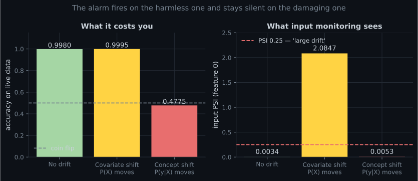
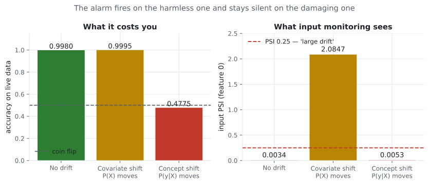
Read those two rows again.

Covariate shift set off a screaming alarm and cost nothing. PSI 2.0847 against a conventional “large drift” threshold of 0.25 — and accuracy was 0.9995, marginally better than the no-drift case. Because $P(y \mid X)$ never changed, the model was still right about the new inputs. Retraining here would have been work for no benefit, and if you had auto-retrained on a small recent window you might well have made things worse.

Concept shift was invisible and halved accuracy. PSI 0.0053 — as stable as the no-drift baseline — while the model fell to 0.4775. Every input looked exactly as expected. The answers changed.

So the honest conclusion: input drift monitoring is neither necessary nor sufficient for detecting performance loss. It is still worth having — it is cheap, label-free and catches broken upstream pipelines fast — but it is a smoke detector in one room of the house, and you should not describe it as fire safety.

What the statistics can see

Two standard tests for “has this distribution moved?”

Population Stability Index. Bin the reference sample (usually deciles), compute the proportion of each sample in each bin, and sum a symmetrised log-ratio:

where $r_i$ and $c_i$ are the reference and current proportions in bin $i$. The conventional read is $< 0.1$ stable, $0.1$–$0.25$ moderate, $> 0.25$ large. Those thresholds are convention, not theory.

Kolmogorov-Smirnov statistic. The largest vertical gap between the two empirical CDFs:

It comes with a p-value, which is both its advantage and its trap.

Measured against a known shift, 4,000 reference rows against 2,000 current:

figureNeither statistic notices a small shift, and both scream at a large onematplotlib

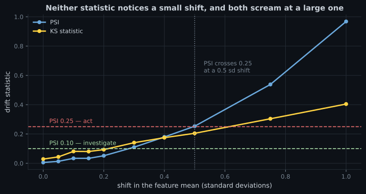
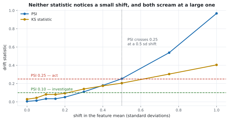
That p-value column is the trap. With enough rows, the KS test rejects any shift. At 0.10 sd the p-value is $4.4 \times 10^{-8}$ — a shift so small that it almost certainly does not affect your model, reported as one of the most statistically significant results you will ever see. Use the statistic, not the p-value, and set the threshold from what your model actually tolerates.

Your dashboard is a picture of the past

The one thing worth monitoring above all others is actual performance. The problem is that performance requires labels, and labels arrive late — sometimes very late.

• Fraud: days to weeks, until a chargeback lands.
• Churn: a month or a quarter, by definition.
• Loan default: months to years.
• Ad clicks: minutes. (This is the lucky case, and it is why ad-tech monitoring looks so different.)

Here is what a 30-day label lag does. Concept drift begins on day 20 and ramps up:

figureConcept drift: invisible to inputs, and 30 days stale in the metricsmatplotlib

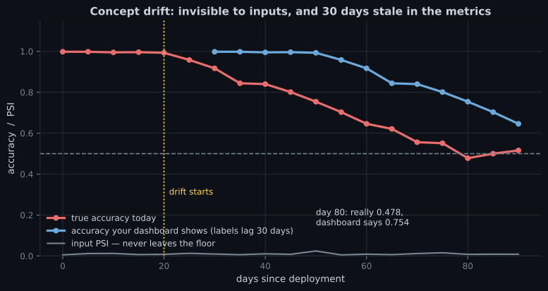
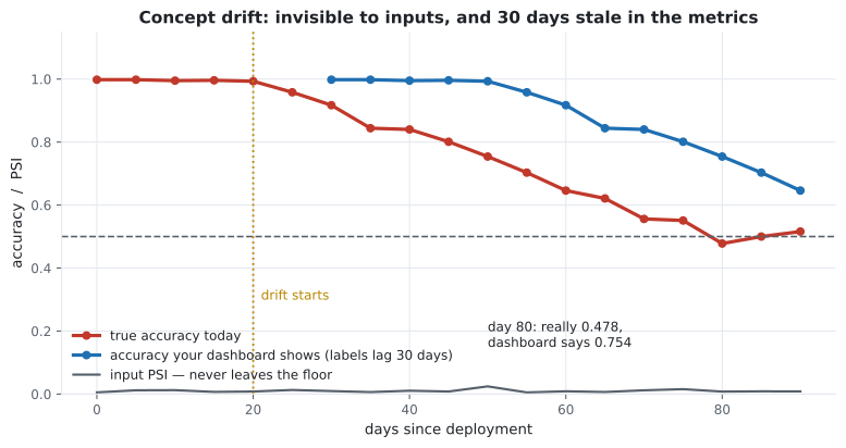
On day 60 the model is at 0.6460 and your dashboard says 0.9170. Input monitoring says everything is fine, because for concept drift it genuinely cannot say otherwise. You are running a substantially broken model with two green lights.

This is not an argument against monitoring. It is an argument for knowing the latency of each signal you rely on:

See it move

Watch the two indicators on the right. Accuracy slides from 1.0000 toward 0.5 as the grey line rotates away from the amber one, and the PSI bar never moves — because the cloud of points is identical throughout. Nothing about the inputs changed. Only the correct answer did.

Prediction drift: the cheap middle ground

The most under-used signal is the distribution of your model’s own output. It needs no labels, arrives immediately, and unlike input monitoring it responds to concept drift — because when the relationship changes, the mix of predictions usually changes with it.

If your fraud model flagged 2.1% of transactions every day for six months and today it flags 7.4%, something happened. You do not know what, and you do not need labels to know it is worth looking at.

import numpy as np
 
 
def psi(reference, current, bins=10):
    """Population Stability Index, binned on the reference deciles."""
    edges = np.quantile(reference, np.linspace(0, 1, bins + 1))
    edges[0], edges[-1] = -np.inf, np.inf
    ref = np.clip(np.histogram(reference, edges)[0] / len(reference), 1e-6, None)
    cur = np.clip(np.histogram(current, edges)[0] / len(current), 1e-6, None)
    return float(((cur - ref) * np.log(cur / ref)).sum())
 
 
def daily_report(reference_X, reference_pred, live_X, live_pred, feature_names):
    """Everything you can compute today, with no labels at all."""
    report = {"n_live": len(live_X), "features": {}}
 
    for j, name in enumerate(feature_names):
        report["features"][name] = {
            "psi": round(psi(reference_X[:, j], live_X[:, j]), 4),
            "mean_shift_sd": round(
                float((live_X[:, j].mean() - reference_X[:, j].mean())
                      / reference_X[:, j].std()), 3),
            "null_rate": round(float(np.isnan(live_X[:, j]).mean()), 4),
        }
 
    # The signal that responds to concept drift without needing labels.
    report["prediction_psi"] = round(psi(reference_pred, live_pred), 4)
    report["positive_rate"] = round(float((live_pred >= 0.5).mean()), 4)
    report["reference_positive_rate"] = round(float((reference_pred >= 0.5).mean()), 4)
    return report

import numpy as np
 
 
def psi(reference, current, bins=10):
    """Population Stability Index, binned on the reference deciles."""
    edges = np.quantile(reference, np.linspace(0, 1, bins + 1))
    edges[0], edges[-1] = -np.inf, np.inf
    ref = np.clip(np.histogram(reference, edges)[0] / len(reference), 1e-6, None)
    cur = np.clip(np.histogram(current, edges)[0] / len(current), 1e-6, None)
    return float(((cur - ref) * np.log(cur / ref)).sum())
 
 
def daily_report(reference_X, reference_pred, live_X, live_pred, feature_names):
    """Everything you can compute today, with no labels at all."""
    report = {"n_live": len(live_X), "features": {}}
 
    for j, name in enumerate(feature_names):
        report["features"][name] = {
            "psi": round(psi(reference_X[:, j], live_X[:, j]), 4),
            "mean_shift_sd": round(
                float((live_X[:, j].mean() - reference_X[:, j].mean())
                      / reference_X[:, j].std()), 3),
            "null_rate": round(float(np.isnan(live_X[:, j]).mean()), 4),
        }
 
    # The signal that responds to concept drift without needing labels.
    report["prediction_psi"] = round(psi(reference_pred, live_pred), 4)
    report["positive_rate"] = round(float((live_pred >= 0.5).mean()), 4)
    report["reference_positive_rate"] = round(float((reference_pred >= 0.5).mean()), 4)
    return report

Note mean_shift_sdmean_shift_sd. Reporting a raw mean change is useless across features with different units; dividing by the training standard deviation makes “this feature moved 0.4 sd” comparable everywhere.

Thresholds and what to do

Alerting on every statistically significant change means alerting constantly. Alert on changes big enough to matter.

Two qualifiers on that table. “And the feature matters” does real work — a PSI of 0.4 on a feature with near-zero importance is not worth a retrain. And “sustained” matters because a single bad day is usually a bad day, not drift.

When an alarm fires, in order:

1. Is the pipeline broken? A null rate jumping to 40% is an upstream bug, not drift. Check this first; it is the most common cause and the fastest to fix.
2. Which drift is it? If performance is unchanged, you may have covariate drift that costs nothing — measured at PSI 2.08 with accuracy 0.9995. Verify before acting.
3. Do you have labels? Without them you cannot confirm a performance drop, only suspect one.
4. Retrain on recent data. For concept drift this is the only real fix. Consider weighting recent rows more heavily.
5. Roll back if the retrain is worse. Which requires that you versioned the artefact.

In code

Reproducing the central measurement:

import numpy as np
from sklearn.linear_model import LogisticRegression
 
TRAIN_ANGLE = 45.0
 
 
def stream(n, angle_deg=TRAIN_ANGLE, shift=0.0, seed=1):
    """shift moves P(X); angle_deg moves P(y|X). Independently."""
    rng = np.random.default_rng(seed)
    X = rng.normal(shift, 1, (n, 2))
    a = np.radians(angle_deg)
    w = np.array([np.cos(a), np.sin(a)])
    return X, (X @ w > 0).astype(int)
 
 
X_tr, y_tr = stream(4000, seed=1)
model = LogisticRegression().fit(X_tr, y_tr)
 
for name, (X_live, y_live) in [
    ("no drift        ", stream(2000, seed=2)),
    ("covariate shift ", stream(2000, shift=1.5, seed=3)),
    ("concept shift   ", stream(2000, angle_deg=TRAIN_ANGLE + 90, seed=4)),
]:
    print(f"{name} accuracy {model.score(X_live, y_live):.4f}   "
          f"PSI {psi(X_tr[:, 0], X_live[:, 0]):.4f}")
 
# no drift         accuracy 0.9980   PSI 0.0034
# covariate shift  accuracy 0.9995   PSI 2.0847      <- alarm, no damage
# concept shift    accuracy 0.4775   PSI 0.0053      <- damage, no alarm

import numpy as np
from sklearn.linear_model import LogisticRegression
 
TRAIN_ANGLE = 45.0
 
 
def stream(n, angle_deg=TRAIN_ANGLE, shift=0.0, seed=1):
    """shift moves P(X); angle_deg moves P(y|X). Independently."""
    rng = np.random.default_rng(seed)
    X = rng.normal(shift, 1, (n, 2))
    a = np.radians(angle_deg)
    w = np.array([np.cos(a), np.sin(a)])
    return X, (X @ w > 0).astype(int)
 
 
X_tr, y_tr = stream(4000, seed=1)
model = LogisticRegression().fit(X_tr, y_tr)
 
for name, (X_live, y_live) in [
    ("no drift        ", stream(2000, seed=2)),
    ("covariate shift ", stream(2000, shift=1.5, seed=3)),
    ("concept shift   ", stream(2000, angle_deg=TRAIN_ANGLE + 90, seed=4)),
]:
    print(f"{name} accuracy {model.score(X_live, y_live):.4f}   "
          f"PSI {psi(X_tr[:, 0], X_live[:, 0]):.4f}")
 
# no drift         accuracy 0.9980   PSI 0.0034
# covariate shift  accuracy 0.9995   PSI 2.0847      <- alarm, no damage
# concept shift    accuracy 0.4775   PSI 0.0053      <- damage, no alarm

Scheduled retraining, which handles most drift without any detection at all:

def should_promote(candidate, incumbent, X_recent, y_recent, margin=0.005):
    """Only replace the live model if the challenger is genuinely better."""
    cand = candidate.score(X_recent, y_recent)
    inc = incumbent.score(X_recent, y_recent)
    print(f"candidate {cand:.4f} vs incumbent {inc:.4f}")
    return cand > inc + margin

def should_promote(candidate, incumbent, X_recent, y_recent, margin=0.005):
    """Only replace the live model if the challenger is genuinely better."""
    cand = candidate.score(X_recent, y_recent)
    inc = incumbent.score(X_recent, y_recent)
    print(f"candidate {cand:.4f} vs incumbent {inc:.4f}")
    return cand > inc + margin

The marginmargin is what stops you shipping a new model every week on noise. And note that the comparison is on recent data — scoring both on the original test set would tell you which model is better at the world as it used to be.

Pitfalls

Treating input drift as a performance proxy. Measured: PSI 2.0847 with accuracy 0.9995, and PSI 0.0053 with accuracy 0.4775. It is neither necessary nor sufficient.

Alerting on KS p-values. At 4,000 rows a 0.10 sd shift gives $p = 4.4 \times 10^{-8}$. Use the statistic and a threshold you chose.

Forgetting the label lag. On day 60 the true accuracy was 0.6460 and the dashboard said 0.9170. Know the latency of every signal you trust.

Auto-retraining on every alarm. The covariate-shift case would have triggered a retrain that bought nothing, on a possibly-small recent window.

Not monitoring predictions. It is label-free, immediate, and unlike input monitoring it responds to concept drift.

Alerting on a single bad day. Require the decline to be sustained, or you will train yourself to ignore the alerts.

Monitoring drift without knowing feature importance. A large PSI on an unimportant feature is noise; a moderate PSI on your top feature is not.

Recap

• $P(X)$ moving is covariate drift; $P(y \mid X)$ moving is concept drift; the metric moving is a symptom.
• Input monitoring is neither necessary nor sufficient: PSI 2.0847 with accuracy 0.9995, and PSI 0.0053 with accuracy 0.4775.
• PSI crosses the conventional 0.25 threshold at a 0.5 sd shift. Use the statistic, never the KS p-value.
• A 30-day label lag meant a true accuracy of 0.6460 displayed as 0.9170.
• Prediction distributions are the cheap middle ground — label-free, immediate, and sensitive to concept drift.
• Check the pipeline first, confirm which drift it is, then retrain on recent data with a promotion margin.
• Scheduled retraining solves most drift without needing to detect anything.

🧪 Try It Yourself

Exercise 1 – Implement PSI

Exercise 2 – Separate the two drift types

Exercise 3 – Standardise the shift so features are comparable

Exercise 4 – Watch the dashboard lag behind reality

Exercise 5 – Promote only on a real improvement

Exercise 6 – Implement PSI and calibrate your intuition

Next

That completes Phase 8 and the module. Go back to the phase overview for the practice project, or return to the Machine Learning landing page to see how the twelve phases fit together.