
DBSCAN - Density-Based Clustering
What you’ll learn
Section titled “What you’ll learn”- the definitions of core, border and noise, and the reachability relations built on them
- the full algorithm traced by hand on ten points on a line
- why DBSCAN needs no — and why it cannot be asked for one
- how to choose
epsfrom the k-distance plot instead of guessing - the measured eps sweep: 21 clusters, then 2, then 2, then 1
- DBSCAN against k-means on two datasets: ARI 1.00 vs 0.24, and 0.57 vs 0.94
- the varying-density failure, and why HDBSCAN exists
Intuition
Section titled “Intuition”k-means asks “which centre is this point nearest?” DBSCAN asks a different question entirely: “is this point in a crowd, and can I walk from crowd to crowd without leaving one?”
A cluster, in this view, is a connected region of high density. It has whatever shape the dense region has — a ring, a crescent, a branching filament. And crucially, points in the sparse gaps between clusters belong to nothing. DBSCAN is the only algorithm in this phase that can say “I don’t know” about a point.
Two parameters define “crowd”:
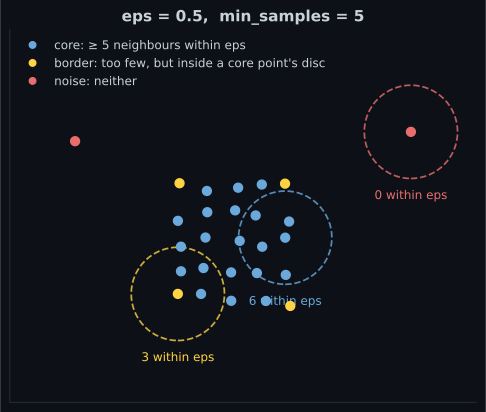
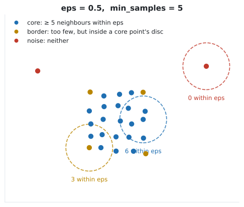
eps() — the radius of the neighbourhood.min_samples— how many points must be inside that radius to count as dense.
Everything else follows mechanically.
  flowchart TD
  P["A point p"] --> Q{"At least min_samples points
within eps of p
(counting p itself)?"}
  Q -->|"yes"| C["CORE point.
Start or extend a cluster;
absorb the whole neighbourhood."]
  Q -->|"no"| R{"Is p within eps
of some core point?"}
  R -->|"yes"| B["BORDER point.
Joins that core point's cluster
but does not expand it."]
  R -->|"no"| N["NOISE.
Label -1. Belongs to nothing."]
The math
Section titled “The math”Write for the -neighbourhood of :
N_\varepsilon(p) = \{\, q \in D : d(p, q) \le \varepsilon \,\}$Note that — scikit-learn counts the point itself, so min_samples=5
means four neighbours plus the point.
Core point. is a core point if
Directly density-reachable. is directly density-reachable from if is a core point and . This relation is not symmetric: a border point is directly reachable from a core point, but not the other way round.
Density-reachable. is density-reachable from if there is a chain where each is directly density-reachable from . Every link except possibly the last must be a core point. This is the transitive closure, and it is what lets a cluster snake around a crescent.
Density-connected. and are density-connected if some core point reaches both. This is symmetric, and it is the relation that actually defines a cluster.
A cluster is a maximal set satisfying:
- Maximality: if and is density-reachable from , then .
- Connectivity: every pair in is density-connected.
Anything in no cluster is noise.
One consequence of these definitions catches people out: a border point can be within of core points from two different clusters. It joins whichever one reaches it first, so its label depends on iteration order. Core points are deterministic; border points are not.
Worked example by hand
Section titled “Worked example by hand”Ten points on a line, with and min_samples = 3:
Step one is to count each neighbourhood, remembering to include the point itself.
| Points within 0.6 (inclusive) | Type | ||
|---|---|---|---|
| 1.0 | 1.0, 1.4 | 2 | border |
| 1.4 | 1.0, 1.4, 1.8 | 3 | core |
| 1.8 | 1.4, 1.8, 2.1 | 3 | core |
| 2.1 | 1.8, 2.1, 2.5 | 3 | core |
| 2.5 | 2.1, 2.5 | 2 | border |
| 6.0 | 6.0 | 1 | noise |
| 9.0 | 9.0, 9.3 | 2 | border |
| 9.3 | 9.0, 9.3, 9.7 | 3 | core |
| 9.7 | 9.3, 9.7, 10.1 | 3 | core |
| 10.1 | 9.7, 10.1 | 2 | border |
Now walk the algorithm:
- Start at 1.0. Only 2 neighbours, not core — set aside for now.
- Move to 1.4. Core. Open cluster 0 and absorb . 1.0 joins as a border point.
- 1.8 is in cluster 0 and is itself core, so absorb — 2.1 joins.
- 2.1 is core, so absorb — 2.5 joins as a border point.
- 2.5 is not core, so the expansion stops. Cluster 0 is .
- 6.0 has one neighbour (itself) and is within of no core point. Noise, label -1.
- 9.3 is core. Open cluster 1, absorb ; 9.7 is core, so absorb . Cluster 1 is .
Final labels, in input order:
Two clusters and one noise point, and at no stage did anything ask how many clusters there should be. The gap at 6.0 is what separates them, and the gap is a property of the data.
See it move
Section titled “See it move”The next sketch makes the reachability chain explicit — click anywhere to drop a seed and watch the cluster flood outward, one core point at a time.
Seed inside one crescent and the flood traces it end to end, then stops — the gap to the other
crescent is wider than eps, so no chain of core points crosses it. Seed on an isolated noise
point and nothing happens at all: it is not core, so it never expands.
eps is the whole ballgame
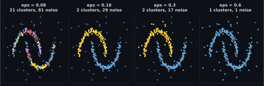
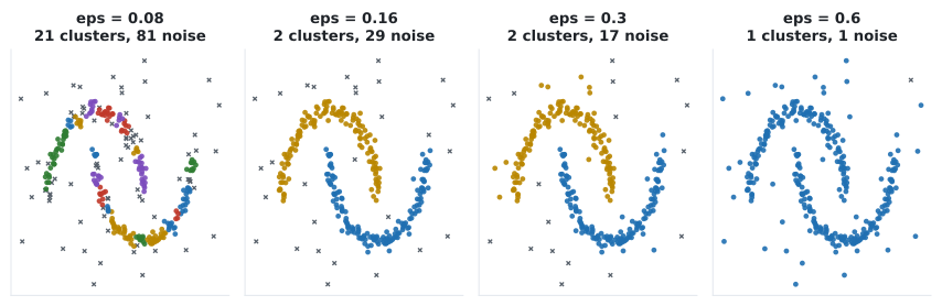
Section titled “eps is the whole ballgame”min_samples is forgiving. eps is not. Here is one dataset — 320 points forming two crescents
plus 40 scattered noise points — under four values:
eps | Clusters found | Points labelled noise |
|---|---|---|
| 0.08 | 21 | 81 |
| 0.16 | 2 | 29 |
| 0.30 | 2 | 17 |
| 0.60 | 1 | 1 |
Too small and the crescents shatter into fragments while a quarter of the data becomes noise. Too large and everything — including the scattered clutter — fuses into a single cluster. The useful range here is roughly 0.15 to 0.35.
By contrast, min_samples barely moves the answer at eps = 0.16:
min_samples | Clusters | Noise |
|---|---|---|
| 3 | 2 | 29 |
| 5 | 2 | 29 |
| 10 | 2 | 30 |
| 20 | 0 | 320 |
Stable until it isn’t: at 20, no point in this dataset has 19 neighbours within 0.16, so
everything is noise. The usual heuristic is min_samples , and is a common
default for features.
Choosing eps from the data
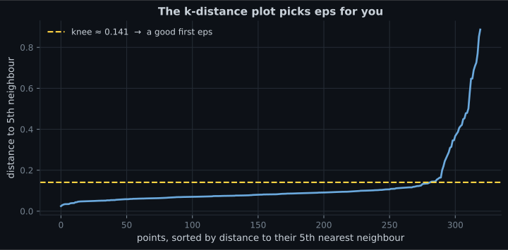
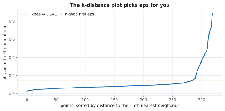
Section titled “Choosing eps from the data”Do not guess. For each point, compute the distance to its -th nearest neighbour (with
min_samples), sort those distances, and plot them. Points inside a cluster have small
-distances; noise points have large ones. The knee of the curve — where it turns sharply
upward — separates the two populations, and its height is a good eps.
On the dataset above, with , the median 5-distance is 0.0818 and the knee sits around 0.1408 — right in the working range the sweep identified.
import numpy as np
from sklearn.neighbors import NearestNeighbors

k = 5                                     # same as min_samples
nn = NearestNeighbors(n_neighbors=k).fit(X)
distances, _ = nn.kneighbors(X)
k_dist = np.sort(distances[:, -1])        # distance to the kth neighbour, sorted

import matplotlib.pyplot as plt
plt.plot(k_dist)
plt.ylabel(f"distance to {k}th nearest neighbour")
plt.xlabel("points, sorted")
plt.show()                                # read eps off the knee
DBSCAN against k-means
Section titled “DBSCAN against k-means”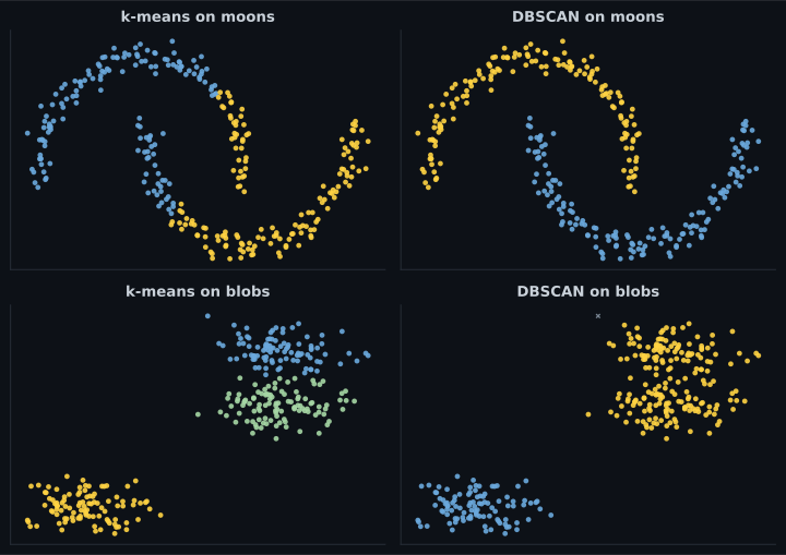
| Dataset | k-means ARI | DBSCAN ARI | Winner |
|---|---|---|---|
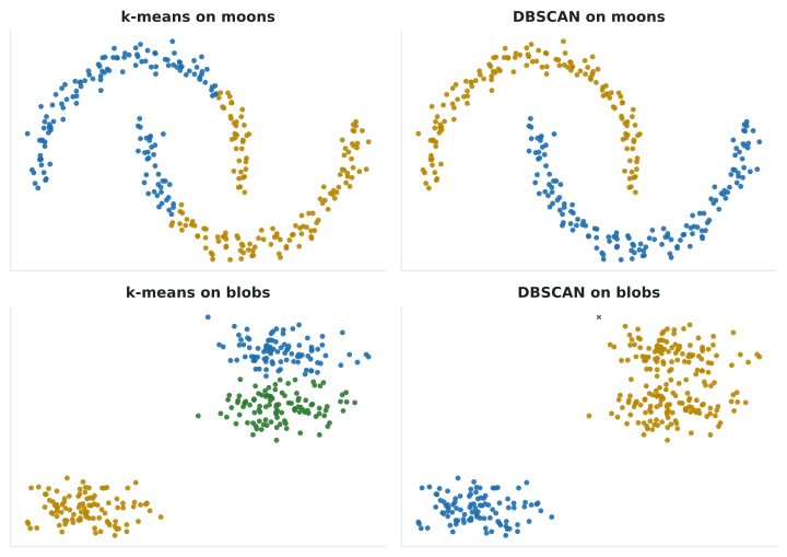
| Two moons | 0.2408 | 1.0000 | DBSCAN, decisively |
| Three blobs (two touching) | 0.9414 | 0.5686 | k-means |
Both results follow directly from the assumptions. k-means draws straight boundaries, which is wrong for crescents and right for separated blobs. DBSCAN follows density, which traces crescents perfectly and cannot separate two blobs whose densities merge where they touch.
The failure mode: varying density
Section titled “The failure mode: varying density”DBSCAN has exactly one global eps. If one genuine cluster is dense and another is sparse, no
single value serves both: pick a small eps and the sparse cluster becomes noise; pick a large one
and the dense clusters merge.
You saw this on the intro page’s third column — the wide cluster dissolved into noise while the tight ones survived.
HDBSCAN fixes this by running DBSCAN at every eps simultaneously and extracting the clusters
that persist over the widest range of scales. It replaces eps with min_cluster_size, which is a
far more interpretable question (“what is the smallest group I care about?”). It is in scikit-learn
from version 1.3 as sklearn.cluster.HDBSCAN.
from sklearn.cluster import DBSCAN, HDBSCAN

db = DBSCAN(eps=0.16, min_samples=5).fit_predict(X)     # 2 clusters, 29 noise
hd = HDBSCAN(min_cluster_size=15).fit_predict(X)        # 2 clusters, 28 noise
On this well-behaved dataset HDBSCAN matches DBSCAN almost exactly — which is the point: you got the same answer without having to find eps first. On varying-density data it wins outright.
OPTICS takes a related approach, producing a reachability plot from which clusterings at many
eps values can be extracted. It is slower and its output takes practice to read; on the same
dataset with default xi=0.05 it returned 21 clusters and 140 noise points, which is a fair
warning that it needs tuning of its own.
In code
Section titled “In code”import numpy as np
from sklearn.cluster import DBSCAN
from sklearn.datasets import make_moons
X, y = make_moons(n_samples=300, noise=0.06, random_state=4)
db = DBSCAN(eps=0.25, min_samples=5).fit(X)
labels = db.labels_
n_clusters = len(set(labels)) - (1 if -1 in labels else 0)
print("clusters", n_clusters) # 2
print("noise ", int((labels == -1).sum())) # 0
# Which points are core? DBSCAN tells you directly.
core_mask = np.zeros(len(X), dtype=bool)
core_mask[db.core_sample_indices_] = True
print("core ", int(core_mask.sum()))
print("border ", int(((labels != -1) & ~core_mask).sum()))Three things to know about the API:
Noise is label -1. Never call len(set(labels)) and assume that is the cluster count; use the
subtraction above. And never feed -1 into silhouette_score without deciding what it means — the
usual choice is to score only the clustered points.
There is no predict. DBSCAN defines clusters relative to the training set. To label a new
point, the standard workaround is to assign it to the cluster of its nearest core sample, if one is
within eps:
import numpy as np
from sklearn.neighbors import NearestNeighbors

def dbscan_assign(db, X_train, X_new, eps):
    """Assign new points to the cluster of the nearest core sample, else noise."""
    cores = X_train[db.core_sample_indices_]
    core_labels = db.labels_[db.core_sample_indices_]
    dist, idx = NearestNeighbors(n_neighbors=1).fit(cores).kneighbors(X_new)
    out = core_labels[idx[:, 0]]
    out[dist[:, 0] > eps] = -1
    return out
Scale first, and use an index. With a ball tree or KD tree, DBSCAN runs in ; without one it degrades to . scikit-learn picks an index automatically for low-dimensional Euclidean data, but in high dimensions the index stops helping and you are back to quadratic.
pch.algoApi sklearn.cluster.DBSCAN
pch.algoAssumes
- Clusters are regions of higher density than the gaps between them
- All clusters have roughly the SAME density — one global eps must serve all of them
- The distance metric is meaningful and the features are scaled
- Density is measurable, which fails in very high dimensions
pch.algoCost
- pch.algoTrain
O(n log n) with a spatial index; O(n^2) without one or in high dimensions- pch.algoPredict
not supported — assign to the nearest core sample manually- pch.algoMemory
O(n p) with an index; O(n^2) if a full distance matrix is precomputed
eps — neighbourhood radius; N_eps(p) — the eps-neighbourhood of p, including p; min_samples — density threshold
pch.algoHyperparams
-
epsdefault 0.5 The whole answer. 21 clusters at 0.08, 1 cluster at 0.60 on the same data. Read it off the k-distance knee. -
min_samplesdefault 5 Density threshold, counting the point itself. Stable across 3-10 here; use at least p+1. -
metricdefault 'euclidean' Any metric, including 'precomputed' if you supply a distance matrix. -
algorithmdefault 'auto' Picks ball_tree, kd_tree or brute. The index is what buys you O(n log n).
pch.algoReachFor
- Clusters have arbitrary shapes — crescents, rings, filaments
- You do not know k and do not want to pick one
- The data has outliers you want identified rather than absorbed
- Cluster densities are broadly comparable
pch.algoLookElsewhere
- Cluster densities differ a lot — use HDBSCAN instead
- Dimensionality is high; all pairwise distances converge and density loses meaning
- You need to label streaming or unseen points
- You need every point assigned to something
Pitfalls
Section titled “Pitfalls”Guessing eps. The sweep above went 21 → 2 → 2 → 1 clusters over a four-fold range. Always plot the k-distance curve first.
Forgetting -1 in the cluster count. len(set(labels)) counts noise as a cluster. It also
breaks any code that indexes an array by label.
Not scaling. eps is a single radius in the raw feature space. If one column runs to 50,000 and another to 1, eps is entirely determined by the first.
Expecting predict. It does not exist, and the nearest-core-sample workaround above is an
approximation you should test before relying on.
Using it in high dimensions. Beyond roughly 10 to 20 features, the distance to the nearest neighbour and to the farthest converge, the k-distance plot flattens out, and there is no knee to read. Reduce dimensions with PCA first — or accept that density-based clustering is the wrong tool.
Treating border-point labels as stable. A border point reachable from two clusters joins whichever the iteration reaches first. Core points are deterministic; border assignments are not.
Applying it to clusters of different density. This is the built-in limitation, not a tuning problem. Reach for HDBSCAN.
Compare
Section titled “Compare”| DBSCAN | HDBSCAN | OPTICS | k-means | |
|---|---|---|---|---|
| Needs k | no | no | no | yes |
| Main parameter | eps | min_cluster_size | min_samples + xi | n_clusters |
| Varying density | fails | handles it | handles it | fails |
| Marks noise | yes | yes | yes | no |
| Deterministic | core points yes, border no | yes | yes | no |
| Speed | fast with an index | moderate | slowest | fastest |
| Can predict | no | approximately | no | yes |
-
With min_samples=5, how many OTHER points must be within eps for a point to be core?
scikit-learn includes the point in its own eps-neighbourhood, so |N_eps(p)| >= 5 means four neighbours plus itself. Off-by-one here shifts every core/border boundary in your result.
pch.quizShowAnswer
B — 4, because the point itself counts toward min_samples — scikit-learn includes the point in its own eps-neighbourhood, so |N_eps(p)| >= 5 means four neighbours plus itself. Off-by-one here shifts every core/border boundary in your result.
-
DBSCAN labels 40% of your data -1. What is the most likely cause?
eps too small means few points reach the min_samples threshold, so almost nothing is core and almost everything falls through to noise. The page's sweep shows exactly this: at eps 0.08, 81 of 320 points became noise and the clusters shattered into 21 fragments.
pch.quizShowAnswer
B — eps is too small for the density of your data — eps too small means few points reach the min_samples threshold, so almost nothing is core and almost everything falls through to noise. The page's sweep shows exactly this: at eps 0.08, 81 of 320 points became noise and the clusters shattered into 21 fragments.
-
Why does DBSCAN have no predict method?
A new point might be core and bridge two clusters that were previously separate — which would change the training-set labels too. There is no consistent way to label a new point without refitting, so the API refuses rather than lying.
pch.quizShowAnswer
B — Clusters are defined by density-connectivity within the training set, so adding a point could legitimately merge two existing clusters — A new point might be core and bridge two clusters that were previously separate — which would change the training-set labels too. There is no consistent way to label a new point without refitting, so the API refuses rather than lying.
-
One of your genuine clusters is dense and another is sparse. What happens with DBSCAN?
This is DBSCAN's structural limitation, not a tuning failure — there is one global eps. HDBSCAN was built for exactly this: it runs across all eps values and keeps the clusters that persist longest.
pch.quizShowAnswer
B — No single eps works: small eps makes the sparse cluster noise, large eps merges the dense ones — This is DBSCAN's structural limitation, not a tuning failure — there is one global eps. HDBSCAN was built for exactly this: it runs across all eps values and keeps the clusters that persist longest.
-
DBSCAN scored ARI 1.00 on two moons and 0.57 on three blobs, where k-means scored 0.24 and 0.94. What is the lesson?
k-means assumes straight boundaries between round clusters; DBSCAN assumes clusters are connected dense regions. On the blobs, two clusters nearly touch, so their densities join and DBSCAN merges them. Match the algorithm to the geometry, not to a reputation.
pch.quizShowAnswer
C — Each algorithm wins exactly where its shape assumption holds; neither dominates — k-means assumes straight boundaries between round clusters; DBSCAN assumes clusters are connected dense regions. On the blobs, two clusters nearly touch, so their densities join and DBSCAN merges them. Match the algorithm to the geometry, not to a reputation.
🧪 Try It Yourself
Section titled “🧪 Try It Yourself”Exercise 1 – Core, border and noise by hand
Section titled “Exercise 1 – Core, border and noise by hand”Exercise 2 – Confirm it against sklearn
Section titled “Exercise 2 – Confirm it against sklearn”Exercise 3 – Sweep eps and watch it break
Section titled “Exercise 3 – Sweep eps and watch it break”Exercise 4 – Read eps off the k-distance curve
Section titled “Exercise 4 – Read eps off the k-distance curve”Exercise 5 – Where each algorithm wins
Section titled “Exercise 5 – Where each algorithm wins”- A point is core if its eps-neighbourhood (including itself) holds at least
min_samplespoints, border if it is inside a core point’s disc, noise otherwise. - A cluster is a maximal density-connected set. That definition needs no and imposes no shape.
- The hand trace on ten points gave labels
[0 0 0 0 0 -1 1 1 1 1]— two clusters, one noise point. epsis the model: 21 clusters at 0.08, 2 at 0.16 and 0.30, 1 at 0.60 on identical data.min_samplesis stable from 3 to 10 and then collapses everything to noise at 20.- Choose eps from the k-distance knee: 0.1408 here, and the sweep confirmed the range.
- DBSCAN beat k-means 1.00 to 0.24 on moons and lost 0.57 to 0.94 on touching blobs.
- One global eps cannot serve clusters of different density. HDBSCAN removes that limitation
and replaces eps with
min_cluster_size. - There is no
predict, noise is label-1, and high dimensions destroy the notion of density.
Exercise 6 – Sweep eps and watch the model change species
Section titled “Exercise 6 – Sweep eps and watch the model change species”Anomaly Detection with Isolation Forests — DBSCAN found outliers as a side effect of clustering. The next page makes finding them the whole objective, and does it in a way that gets faster as the data gets bigger.
pch.coffeeTagline
pch.coffeeCtapch.feedbackHeading
pch.feedbackSubheading