What you’ll learn

• why random sampling beats a grid at the same budget, with the geometric argument
• the probability formula behind “59 draws”, derived
• sampling from distributions rather than lists, and which distribution to use
• a head-to-head on real data where random search wins with identical cost
• when a grid is still the right choice
• successive halving, which beats both when fits are expensive

Intuition

A grid search spends its budget on the product of the hyperparameter values. With 6 values of CC and 6 of gammagamma you get 36 fits — but only 6 distinct values of each. If gammagamma turns out not to matter, you paid 36 fits to try 6 values of the one parameter that did.

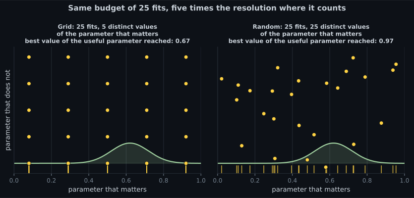
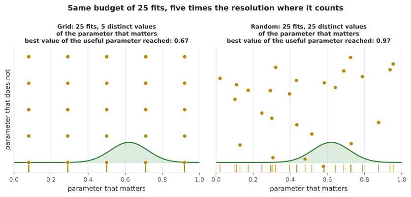
Random search samples each combination independently. Thirty-six draws give you 36 distinct values of every hyperparameter. If only one matters, you explored it six times more thoroughly for the same money.

figureTwenty-five fits eachmatplotlib

Reading the plot

1. Both panels cost exactly 25 fits. This is not a more-compute argument.
2. The grid tries 5 distinct values of the useful parameter. The other 20 fits are repeats along an axis that changes nothing.
3. Random search tries 25 distinct values. Its best landed at 0.97 of the peak against the grid’s 0.67.
4. The grid’s failure is structural, not unlucky. Any grid wastes resolution on parameters that do not matter, and you rarely know in advance which those are.

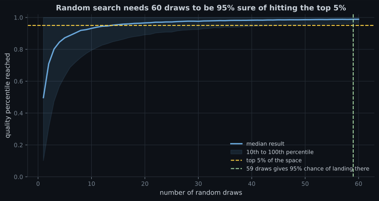
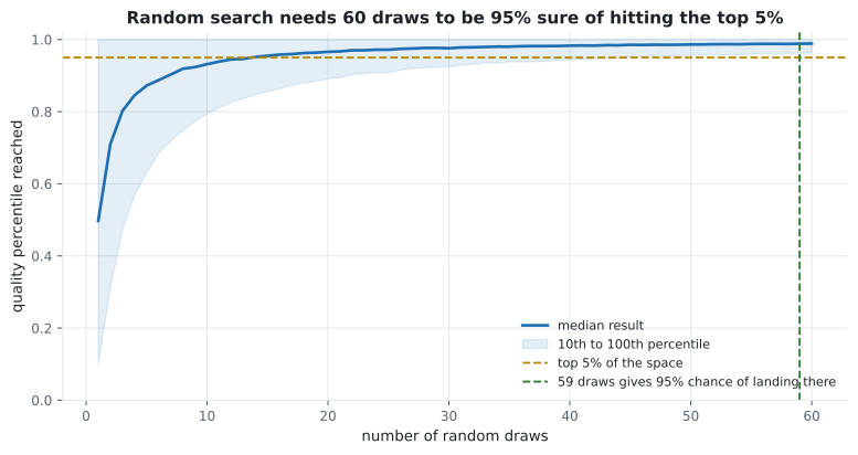
The math

Suppose the top 5% of the hyperparameter space would be “good enough”. A single random draw misses it with probability 0.95. Draws are independent, so $n$ draws all miss with probability $0.95^n$, and:

Solving for the number of draws needed to reach confidence $c$:

With $p = 0.05$ and $c = 0.95$:

The result does not depend on the number of hyperparameters. Fifty-nine draws give 95% confidence of landing in the top 5% whether you are tuning 2 hyperparameters or 20. A grid covering 20 hyperparameters at even 3 values each is $3^{20} \approx 3.5$ billion combinations.

figureDiminishing returns, quantifiedmatplotlib

Worked example by hand

You have 6 hyperparameters and want 5 values of each.

Step 1 — the grid.

At 2 seconds per fit that is 43 hours.

Step 2 — random search at 60 draws.

Step 3 — what each buys. The grid guarantees the best point in the grid. Random search gives 95% confidence of landing in the top 5% of the continuous space — including values no grid contained.

Step 4 — the ratio. 260 times less compute, for a probabilistic rather than exhaustive guarantee. On any real problem where the score surface is smooth, that is the better trade.

Sampling from distributions

Random search’s real advantage over a grid is not randomness, it is continuity. Give it a distribution instead of a list and it can propose values no grid contained:

from scipy.stats import loguniform, randint, uniform
 
param_distributions = {
    # multiplicative parameters: log-uniform, so each decade is equally likely
    "svc__C": loguniform(1e-2, 1e3),
    "svc__gamma": loguniform(1e-4, 1e1),
    # counts: integer uniform
    "rf__n_estimators": randint(50, 500),
    "rf__max_depth": randint(3, 30),
    # genuinely linear parameters: plain uniform
    "rf__max_features": uniform(0.1, 0.8),      # loc=0.1, scale=0.8 -> [0.1, 0.9]
    # categorical: a plain list still works
    "svc__kernel": ["rbf", "poly", "sigmoid"],
}

from scipy.stats import loguniform, randint, uniform
 
param_distributions = {
    # multiplicative parameters: log-uniform, so each decade is equally likely
    "svc__C": loguniform(1e-2, 1e3),
    "svc__gamma": loguniform(1e-4, 1e1),
    # counts: integer uniform
    "rf__n_estimators": randint(50, 500),
    "rf__max_depth": randint(3, 30),
    # genuinely linear parameters: plain uniform
    "rf__max_features": uniform(0.1, 0.8),      # loc=0.1, scale=0.8 -> [0.1, 0.9]
    # categorical: a plain list still works
    "svc__kernel": ["rbf", "poly", "sigmoid"],
}

Head to head

Same model, same data, same budget of 36 combinations:

import numpy as np
from scipy.stats import loguniform
from sklearn.datasets import load_breast_cancer
from sklearn.model_selection import GridSearchCV, RandomizedSearchCV
from sklearn.pipeline import make_pipeline
from sklearn.preprocessing import StandardScaler
from sklearn.svm import SVC
 
X, y = load_breast_cancer(return_X_y=True)
pipe = make_pipeline(StandardScaler(), SVC())
 
grid = GridSearchCV(
    pipe,
    {"svc__C": np.logspace(-2, 3, 6), "svc__gamma": np.logspace(-4, 1, 6)},
    cv=5, n_jobs=-1,
).fit(X, y)
 
random = RandomizedSearchCV(
    pipe,
    {"svc__C": loguniform(1e-2, 1e3), "svc__gamma": loguniform(1e-4, 1e1)},
    n_iter=36, cv=5, random_state=0, n_jobs=-1,
).fit(X, y)
 
print(f"grid    {grid.best_score_:.4f}  {grid.best_params_}")
# grid    0.9789  {'svc__C': 10.0, 'svc__gamma': 0.01}
print(f"random  {random.best_score_:.4f}  "
      f"{ {k: round(v, 5) for k, v in random.best_params_.items()} }")
# random  0.9807  {'svc__C': 7.09551, 'svc__gamma': 0.0156}

import numpy as np
from scipy.stats import loguniform
from sklearn.datasets import load_breast_cancer
from sklearn.model_selection import GridSearchCV, RandomizedSearchCV
from sklearn.pipeline import make_pipeline
from sklearn.preprocessing import StandardScaler
from sklearn.svm import SVC
 
X, y = load_breast_cancer(return_X_y=True)
pipe = make_pipeline(StandardScaler(), SVC())
 
grid = GridSearchCV(
    pipe,
    {"svc__C": np.logspace(-2, 3, 6), "svc__gamma": np.logspace(-4, 1, 6)},
    cv=5, n_jobs=-1,
).fit(X, y)
 
random = RandomizedSearchCV(
    pipe,
    {"svc__C": loguniform(1e-2, 1e3), "svc__gamma": loguniform(1e-4, 1e1)},
    n_iter=36, cv=5, random_state=0, n_jobs=-1,
).fit(X, y)
 
print(f"grid    {grid.best_score_:.4f}  {grid.best_params_}")
# grid    0.9789  {'svc__C': 10.0, 'svc__gamma': 0.01}
print(f"random  {random.best_score_:.4f}  "
      f"{ {k: round(v, 5) for k, v in random.best_params_.items()} }")
# random  0.9807  {'svc__C': 7.09551, 'svc__gamma': 0.0156}

Random search wins, at identical cost. Not because randomness is magic, but because it found $C = 7.096$ and $\gamma = 0.0156$ — values that were not on the grid and could not have been. The grid’s best cell was the nearest lattice point to a better answer sitting between the lines.

This is a single comparison and would not always go this way. The general claim is weaker and still useful: at equal budget, random search is at least competitive, and its advantage grows with the number of hyperparameters.

See it move

Both searchers get the same budget on the same hidden score surface. Watch which one finds the bright region first.

When to prefer which

The standard workflow uses both: a wide random search to find the promising region, then a small grid around the winner to refine it.

Successive halving

When each fit is expensive, most of the budget goes on combinations that were obviously bad after a tenth of the data:

from sklearn.experimental import enable_halving_search_cv  # noqa: F401
from sklearn.model_selection import HalvingRandomSearchCV
 
search = HalvingRandomSearchCV(
    pipe, param_distributions,
    factor=3,             # keep the best third at each round
    resource="n_samples", # the resource being increased is training rows
    random_state=0, n_jobs=-1,
).fit(X, y)

from sklearn.experimental import enable_halving_search_cv  # noqa: F401
from sklearn.model_selection import HalvingRandomSearchCV
 
search = HalvingRandomSearchCV(
    pipe, param_distributions,
    factor=3,             # keep the best third at each round
    resource="n_samples", # the resource being increased is training rows
    random_state=0, n_jobs=-1,
).fit(X, y)

Round 1 evaluates many candidates on a small subset; the best third survive to round 2 with three times the data, and so on. Most candidates are eliminated cheaply, and the survivors get evaluated properly. Note the enable_halving_search_cvenable_halving_search_cv import — the estimator is still experimental.

Picking a search strategy

  flowchart TD
  A["How many hyperparameters,
and how expensive is one fit?"] --> B{"Any continuous
parameters?"}
  B -->|"yes -- C, alpha,
learning_rate"| R["Random search.
A grid cannot express
values between its points."]
  B -->|"no, all discrete"| C{"Size of the
full product?"}
  C -->|"under ~50 combinations"| G["Grid search.
Exhaustive and cheap."]
  C -->|"hundreds or more"| D{"Is one fit
expensive?"}
  D -->|"seconds"| R
  D -->|"minutes or more"| H["Successive halving.
Eliminate on a subset,
promote the survivors."]
  R --> S{"Did the winner sit at
the edge of a range?"}
  S -->|"yes"| W["Widen that range
and search again --
the optimum is outside."]
  S -->|"no"| N["Narrow grid around
the winner to refine."]
  H --> N
  G --> V["Report the CV spread,
not only the best mean."]
  N --> V
  W --> R

The edge check in that flow is the step people skip. A random search whose best CC is the largest value it sampled has not found an optimum, it has found the boundary of the box you drew — and the fix is to redraw the box, not to accept the number.

Pitfalls

🧪 Try It Yourself

Exercise 1 – Grid size against search budget

Exercise 2 – Derive the 59

Exercise 3 – Sample from distributions

Exercise 4 – Run the head-to-head

Exercise 5 – Choose the strategy

Recap

• A $5\times5$ grid tries 5 distinct values per parameter; 25 random draws try 25. When only one parameter matters, that is five times the resolution where it counts.
• $P(\text{hit top } p) = 1 - (1-p)^n$, so 59 draws give 95% confidence of the top 5% — independent of how many hyperparameters there are.
• Sample multiplicative parameters from loguniformloguniform, counts from randintrandint, proportions from uniformuniform, choices from a list.
• Head to head at 36 combinations: grid 0.9789, random 0.9807 — because random could propose $C = 7.096$ and the grid could not.
• Grid for one or two discrete hyperparameters; random for three or more or anything continuous; successive halving when fits are expensive.
• best_score_best_score_ is still optimistic. Nested CV or a held-out test set remains the honest number.

Exercise 6 – How many draws do you actually need?

Next

Continue to The ML Pipeline - Automating the Workflow — everything in this phase assumed a pipeline; this page makes it the reproducible unit you tune, save and ship.